The Bang-Bang Motion Profile
Prerequisites- None
When designing robots that physically move, a common task is for them to move from one point to another; often as fast as possible.
In this article, we will introduce the time optimal bang-bang motion profile and derive an equation that computes the time required to complete a move from one point to another given the distance to move $\Delta x$, the acceleration $a$, and the target velocity $v_t$.
Kinematic Equations
We will need the below two equations. For a motion with constant acceleration, these equations relate travel distance with start/end velocity, acceleration, and travel time:
$$v_f^2 = v_i^2 + 2a\Delta x \: [1]$$
$$\Delta x = v_it + \frac{1}{2}at^2 \:[2]$$
where $\Delta x$ is the travel distance, $t$ is the travel time, $v_i$ is the initial velocity, $v_f$ is the final velocity, and $a$ is the acceleration. We will not derive these equations in this article.
Constant Velocity Motion Profile
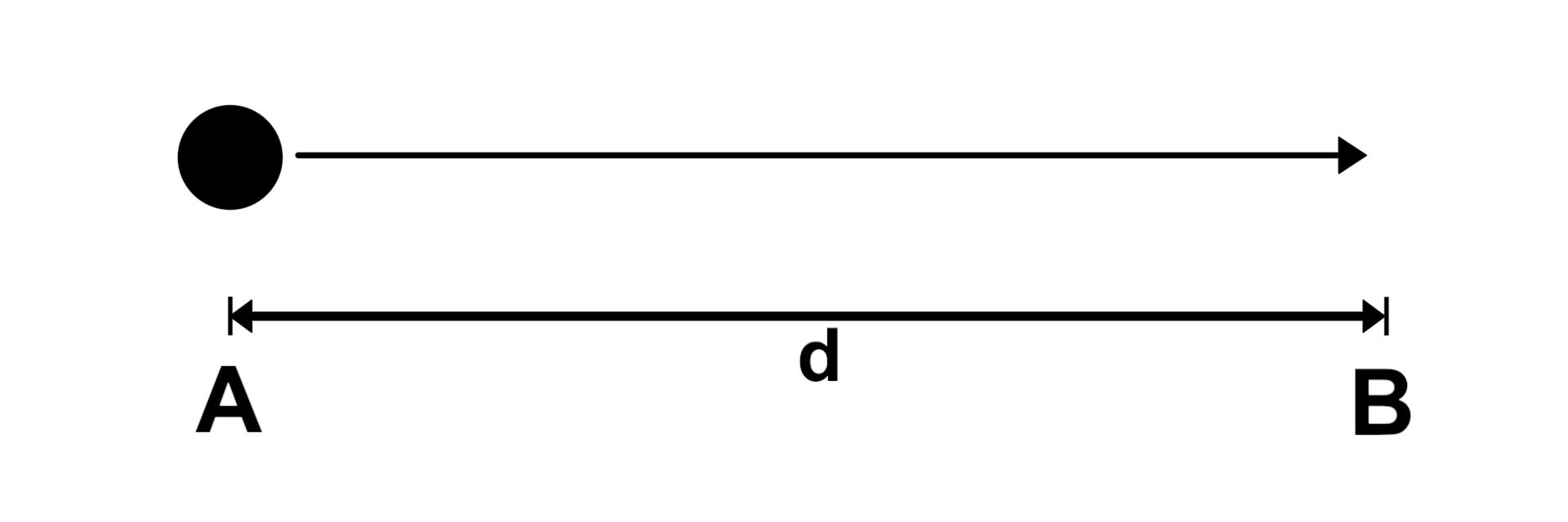
An intuitive proposal for a motion profile is to instantaneously modify the velocity of the point (from a stop to target velocity $v_t$), move it at constant velocity between points $a$ and $b$, then instantaneously bring it to a stop.
Figure 2: The constant velocity motion profile is time efficient.
Unfortunately, it is not physically possible to instantaneously transition a physical robot from stationary to moving at some velocity. A force must be applied to cause the object's speed to change via acceleration per the relationship:
$$F = ma$$
Bang Bang Motion Profile
The bang-bang motion profile conforms to physics by applying an initial acceleration until a target velocity is achieved and then applying a deceleration to slow the robot down at the end point.
Figure 3: The bang-bang motion profile is the most time optimal, physically possible motion profile.
The difference between the bang-bang and the constant velocity profile is a bit subtle. To help accentuate their differences, they are compared below; bang bang on top and constant velocity on bottom.
Figure 4: Constant velocity and bang-bang motion profiles compared against each other.
The bang-bang motion profile takes two different forms; trapezoidal and triangular.
Trapezoidal Motion Profile
The trapezoidal motion profile occurs when the distance, velocity, and acceleration are sufficient to permit the robot to reach the target velocity and travel at that velocity for an amount of time before it needs to begin decelerating.
The trapezoidal motion profile has three stages.
- Accelerate to target velocity, $v_t$
- Travel at the target constant velocity, $v_t$
- Decelerate and stop at the target position
The below three plots of acceleration|time, velocity|time, and position|time demonstrate this motion profile.
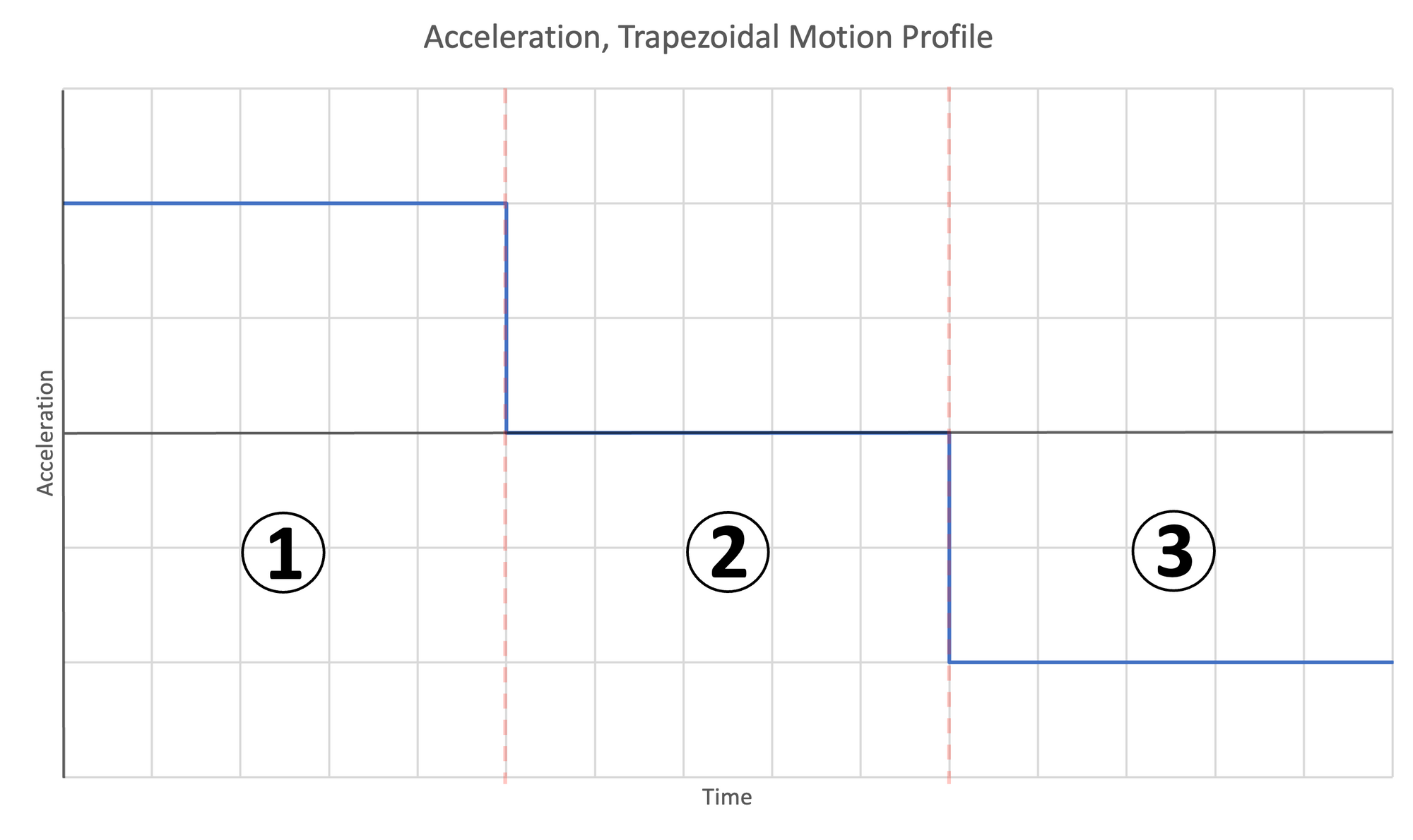
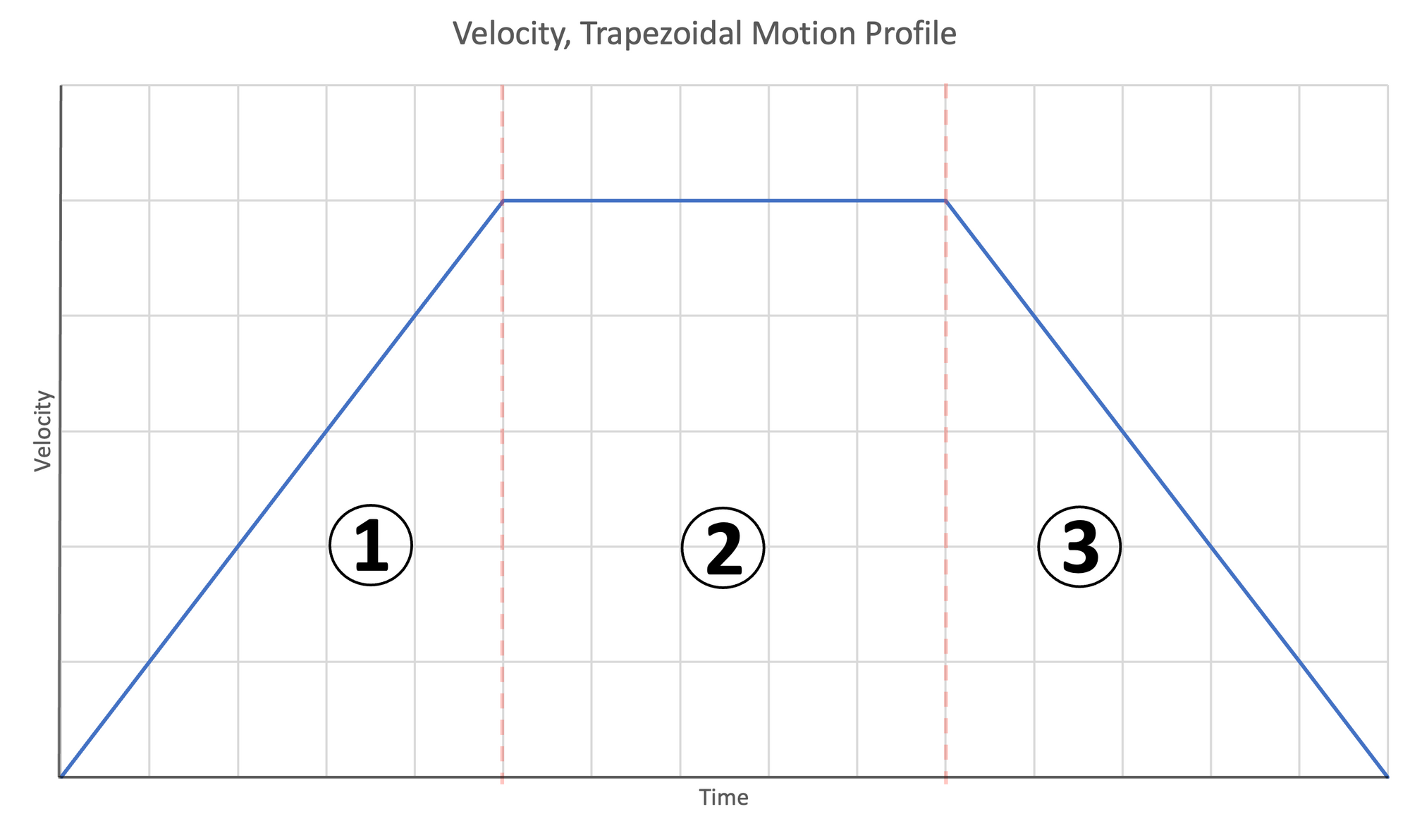
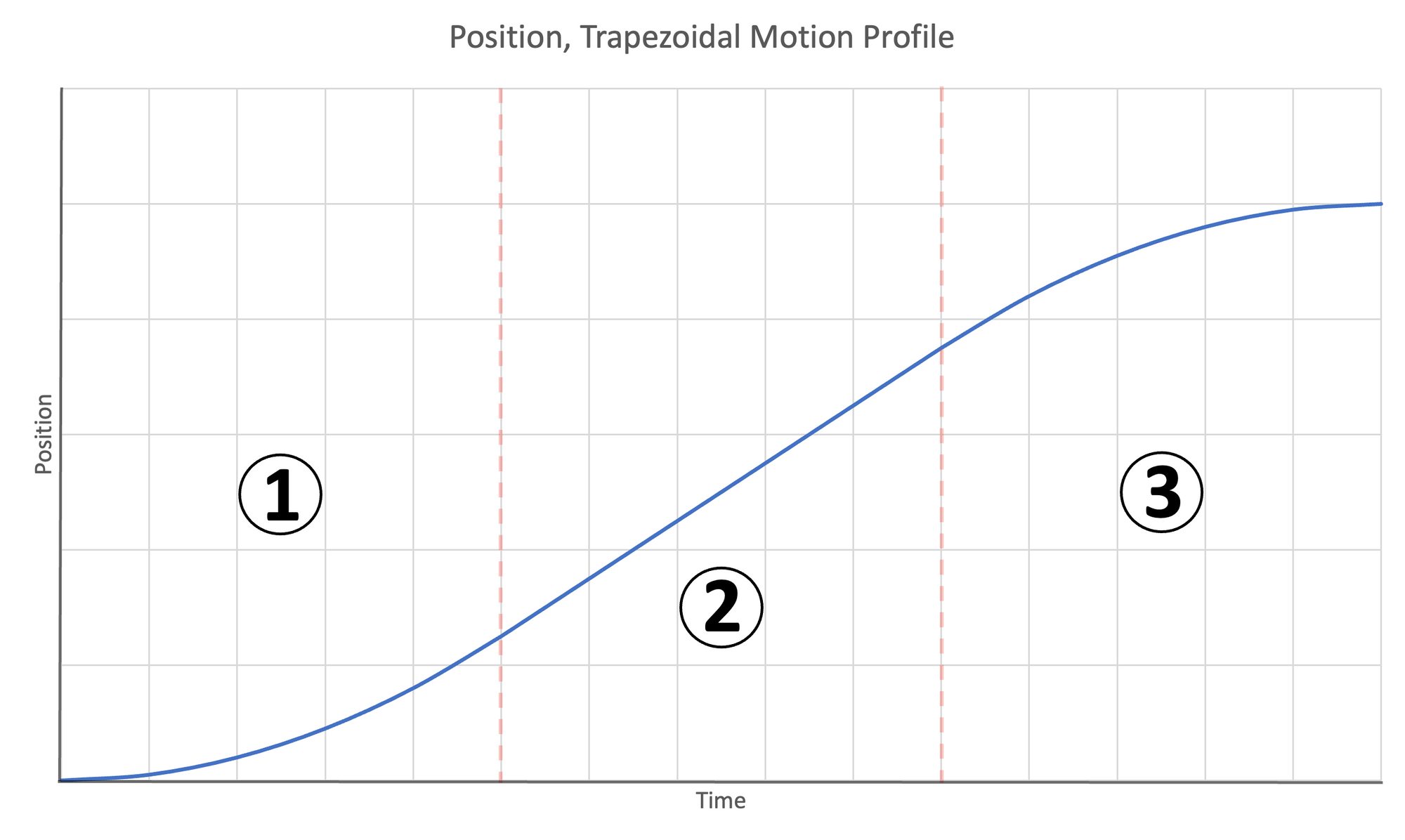
Figure 5: Motion profiles for trapezoidal motion | Left- Acceleration | Center- Velocity | Right- Position
Each stage takes a corresponding amount of time $t_1$, $t_2$, $t_3$ and the total time for the motion is given by adding the times of all stages:
$$t_T = t_1 + t_2 + t_3$$
Stages 1 and 3 are closely related. The accelerations have the same magnitude (though opposite directions), the start and end velocities are flipped, and both stages require the same time and distance to complete, which yields:
$$t_1 = t_3$$
Proof that Stage1 and Stage 3 Require Equal Time and Distances to Complete (A)
Recall our two kinematic equations:
$$v_f^2 = v_i^2 + 2a\Delta x \: [1]$$
$$\Delta x = v_it + \frac{1}{2}at^2 \:[2]$$
Stage 1 has the following properties:
$$v_i = 0,\: v_f = v_t,\: a = a$$
Substituting the properties of stage 1 into kinematic equation $[1]$, we obtain:
$$v_f^2 = v_i^2 + 2a\Delta x_1 \: [1]$$
$$\downarrow$$
$$v_t^2 = 2a\Delta x_1$$
$$\downarrow$$
$$\Delta x_1 = \frac{v_t^2}{2a}\: [A1]$$
Stage 3 has the following properties:
$$v_i = v_t,\: v_f = 0,\: a = -a$$
Substituting the properties of stage 3 into kinematic equation $[1]$, we obtain:
$$v_f^2 = v_i^2 + 2a\Delta x_3 \: [1]$$
$$\downarrow$$
$$0 = v_t^2 - 2a\Delta x_3$$
$$\downarrow$$
$$\Delta x_3 = \frac{v_t^2}{2a}\: [A2]$$
Note that equations $[A1]$ and $[A2]$ are equal to each other, which demonstrates that $\Delta x_1 = \Delta x_3$. Stages 1 and 3 require the same distance to complete.
Substituting the properties of stage 1 into kinematic equation $[2]$, we obtain:
$$\Delta x = v_it + \frac{1}{2}at^2 \:[2]$$
$$\downarrow$$
$$\Delta x_1 = (0)t_1 + \frac{1}{2}at_1^2 $$
$$\downarrow$$
$$t_1 = \sqrt{\frac{2\Delta x_1}{a}}$$
Substituting in $\Delta x_1 = \frac{v_t^2}{2a}$ into the above:
$$t_1 = \sqrt{\frac{2\frac{v_t^2}{2a}}{a}}$$
$$\downarrow$$
$$t_1 = \sqrt{\frac{v_t^2}{a^2}}$$
$$\downarrow$$
$$t_1 = \frac{v_t}{a}\:[A3]$$
Substituting the properties of stage 3 into kinematic equation $[2]$, we obtain:
$$\Delta x = v_it + \frac{1}{2}at^2 \:[2]$$
$$\downarrow$$
$$\Delta x_3 = v_t t_3 - \frac{1}{2}at_3^2 $$
$$\downarrow$$
$$0 = \frac{1}{2}at_3^2 - v_t t_3 + \Delta x_3$$
Using the quadratic formula to solve for $t$, we obtain:
$$t_3 = \frac{v_t \pm \sqrt{v_t^2-4\frac{1}{2}a\Delta x_3}}{2\frac{1}{2}a}$$
$$\downarrow$$
$$t_3 = \frac{v_t \pm \sqrt{v_t^2-2a\Delta x_3}}{a}$$
$$\downarrow$$
$$t_3 = \frac{v_t}{a} \pm \frac{1}{a}\sqrt{v_t^2-2a\Delta x_3}$$
$$\downarrow$$
$$t_3 = \frac{v_t}{a} \pm \sqrt{\frac{v_t^2}{a^2}-\frac{2a\Delta x_3}{a^2}}$$
$$\downarrow$$
$$t_3 = \frac{v_t}{a} \pm \sqrt{\frac{v_t^2}{a^2}-\frac{2\Delta x_3}{a}}$$
Substituting in $\Delta x_3 = \frac{v_t^2}{2a}$ into the above:
$$t_3 = \frac{v_t}{a} \pm \sqrt{\frac{v_t^2}{a^2}-\frac{2\frac{v_t^2}{2a}}{a}}$$
$$\downarrow$$
$$t_3 = \frac{v_t}{a} \pm \sqrt{\frac{v_t^2}{a^2}-\frac{v_t^2}{a^2}}$$
$$\downarrow$$
$$t_3 = \frac{v_t}{a}\: [A4]$$
Note that equations $[A3]$ and $[A4]$ are equal to each other, which demonstrates that $t_1 = t_3$. Stages 1 and 3 require the same time to complete.
Substitutting this into into the total time equation:
$$t_T = t_1 + t_2 + t_1$$
$$\downarrow$$
$$t_T = 2t_1 + t_2\:[3]$$
The time required for stage one is given by:
$$t_1 = \frac{v_t}{a}\: [4]$$
Proof of Time for Stage 1 of Trapezoidal Motion (B)
For stage 1 of the trapezoidal motion profile, $v_{i} = 0$, $v_{f} = v_t$, and $a = a$. Substituting the stage 1 parameters into kinematic equation $[1]$, we obtain:
$$v_f^2 = v_i^2 + 2a\Delta x \: [1]$$
$$\downarrow$$
$$v_{t}^2 = 2a\Delta x_1$$
$$\downarrow$$
$$\Delta x_1= \frac{v_t^2}{2a}$$
Substituting the stage 1 parameters into kinematic equation $[2]$, we obtain:
$$\Delta x = v_it + \frac{1}{2}at^2 \:[2]$$
$$\downarrow$$
$$\Delta x_1 = (0) t_1 + \frac{1}{2}at_1^2$$
$$\downarrow$$
$$\Delta x_1 = \frac{1}{2}at_1^2$$
$$\downarrow$$
$$t_1 = \sqrt{\frac{2\Delta x_1}{a}}$$
Substituting $\Delta x_1= \frac{v_t^2}{2a}$ into the above equation:
$$t_1 = \sqrt{\frac{2\left(\frac{v_t^2}{2a}\right)}{a}}$$
$$\downarrow $$
$$t_1 = \sqrt{\frac{v_t^2}{a^2}}$$
$$\downarrow $$
$$t_1 = \frac{v_t}{a}$$
The time required for stage 2 is given by:
$$t_2 = \frac{\Delta x_T}{v_t} - \frac{v_t}{a}\:[5]$$
Proof of Time for Trapezoidal Motion, Stage 2 (C)
For stage 2 of the motion profile, the distance traveled is equal to the total distance $\Delta x_T$ minus the distance covered during stages one $\Delta x_1$ and three $\Delta x_3$:
$$\Delta x_2 = \Delta x_T - \Delta x_1 - \Delta x_3 $$
Remember that the distances covered during stages one and three are equal, $\Delta x_1 = \Delta x_3$:
$$\Delta x_2 = \Delta x_T - \Delta x_1 - \Delta x_1 $$
$$\downarrow $$
$$\Delta x_2 = \Delta x_T - 2\Delta x_1 $$
Remember that $\Delta x_1= \frac{v_t^2}{2a}$. Substituting into the above equation:
$$\Delta x_2 = \Delta x_T - 2\left(\frac{v_t^2}{2a}\right)$$
$$\Delta x_2 = \Delta x_T - \frac{v_t^2}{a}\:[C1]$$
Because the point is at constant velocity during stage 2 $(v = v_t)$ and zero acceleration $(a = 0)$, the kinematic equation $[2]$ simplifies to:
$$\Delta x = v_it + \frac{1}{2}at^2 \:[2]$$
$$\downarrow $$
$$\Delta x_2 = v_{t}t_2+ \frac{1}{2}(0)t_2^2$$
$$\downarrow $$
$$\Delta x_2 = v_{t}t_2$$
Substituting $[C1]$ into the above equation:
$$\Delta x_T - \frac{v_t^2}{a} = v_{t}t_2$$
$$\downarrow $$
$$t_2 = \frac{\Delta x_T - \left(\frac{v_t^2}{a}\right)}{v_t} $$
$$\downarrow $$
$$t_2 = \frac{\Delta x_T}{v_t} - \frac{v_t}{a} $$
As given in equation $[3]$, $t_T = 2t_1 + t_2$. Substituting in our solutions for $t_1$ in equation $[4]$ and $t_2$ in equation $[5]$, we obtain:
$$t_T = 2t_1 + t_2$$
$$\downarrow $$
$$t_T = 2\frac{v_t}{a} + \frac{\Delta x_T}{v_t} - \frac{v_t}{a} $$
$$\downarrow $$
$$t_T = \frac{\Delta x_T}{v_t} + \frac{v_t}{a}$$
This is the time required to perform a trapezoidal bang-bang motion. Remember that trapezoidal motion consists of three stages. Since the time/distance for stages 1 and 3 are equal, as long as these stages occupy less than half the total time/distance, there will be space for stage 2 and the motion will be trapezoidal.

After performing the calculations, it is found that the motion is only trapezoidal if the following condition is true:
$$\Delta x_T > \frac{v_t^2}{a}\:[6]$$
Proof of Condition for Trapezoidal Motion (D)
Consider the first kinematic equation for a constant acceleration segment:
$$v_f^2 = v_i^2 + 2a\Delta x\:[1]$$
$$\downarrow $$
$$\frac{v_f^2 - v_i^2}{2a} = \Delta x$$
For this stage, $v_f = v_t$, $v_i = 0$. We can substitute these into the above equation:
$$\frac{v_t^2 - 0^2}{2a} = \Delta x_1$$
$$\downarrow $$
$$\frac{v_t^2}{2a} = \Delta x_1$$
As previously explained, for the motion to be trapezoidal, stage one must complete in less than half the total distance $(\Delta x_1 < \frac{\Delta x_T}{2})$. Substituting the above equation into the condition:
$$\frac{v_t^2}{2a} < \frac{\Delta x_T}{2}$$
$$\downarrow $$
$$\Delta x_T > \frac{v_t^2}{a}$$
Triangular Motion Profile
One alternate possibility to trapezoidal motion is that the distance, acceleration, and target velocity are such that the motion is triangular rather than trapezoidal. This occurs when the time/distance available for stage 2 is reduced to $0$.

In this case, stages 1 and 3 complete, but there is no room for stage 2 because the combination of parameters are such that stage one requires exactly half the total distance. In this case, the total time for the motion is:
$$t_t = t_1 + t_3$$
Similar to the trapezoidal profile, the time/distance for stages 1 and 3 are equal.
$$t_t = t_1 + t_1$$
$$\downarrow$$
$$t_t = 2t_1$$
We can substitute in equation $[4]$, $t_1 = \frac{v_t}{a}$ into the above equation:
$$t_t = 2\frac{v_t}{a}\:[7]$$
As explained above, stage one must complete in half the total distance $x_T$. The constraint that ensures this is met is:
$$\Delta x_T = \frac{v_t^2}{a}\:[8]$$
Proof of Condition for Triangular Motion (E)
Consider the first kinematic equation for a constant acceleration segment:
$$v_f^2 = v_i^2 + 2a\Delta x\:[1]$$
$$\downarrow$$
$$\frac{v_f^2 - v_i^2}{2a} = \Delta x$$
As explained above, stage one must complete in exactly half the total distance $x_T$. For this stage, $v_f = v_t$, $v_i = 0$, and $\Delta x = \frac{\Delta x_T}{2}$. We can substitute these into the above equation:
$$\frac{v_t^2 - 0^2}{2a} = \frac{\Delta x_T}{2}$$
$$\downarrow $$
$$\frac{v_t^2}{a} = \Delta x_T$$
$$\downarrow $$
$$\Delta x_T = \frac{v_t^2}{a}$$
Let us substitute our triangular motion constraint into the solution for the trapezoidal motion profile:
$$t_T = \frac{\Delta x_T}{v_t} + \frac{v_t}{a}$$
$$\downarrow$$
$$t_T = \frac{v_t^2}{av_t} + \frac{v_t}{a}$$
$$\downarrow$$
$$t_T = \frac{v_t}{a} + \frac{v_t}{a}$$
$$\downarrow$$
$$t_T = 2\frac{v_t}{a}\:[9]$$
This result from the trapezoidal equation $[9]$ is identical to the result computed from the triangular motion profile $[7]$! This allows us to write a singular equation that describes the motion time for both kinds of motion:
$$t_T = \frac{\Delta x_T}{v_t} + \frac{v_t}{a} \text{ if } \Delta x_T \ge \frac{v_t^2}{a}\:[10]$$
Acceleration Constrained Triangular Motion Profile
During a bang-bang motion profile, the final alternative is where the combination of parameters results in triangular motion, but the target velocity is not achieved.
The triangular motion profile has two stages:
- Accelerate until half the total travel distance has been covered
- Decelerate and stop at the target position
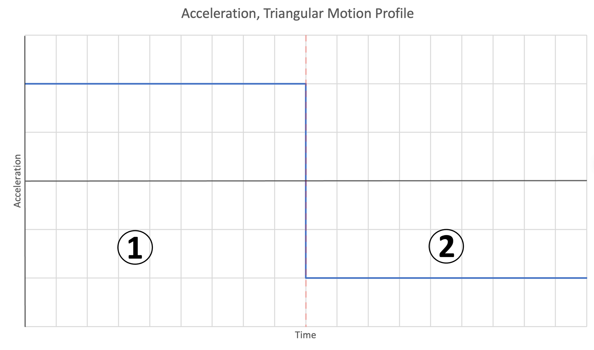
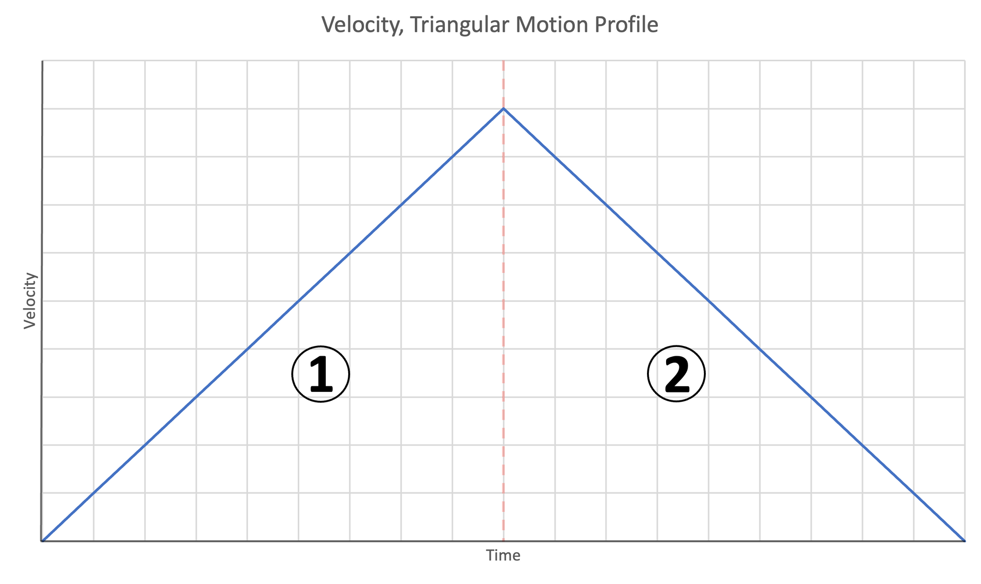
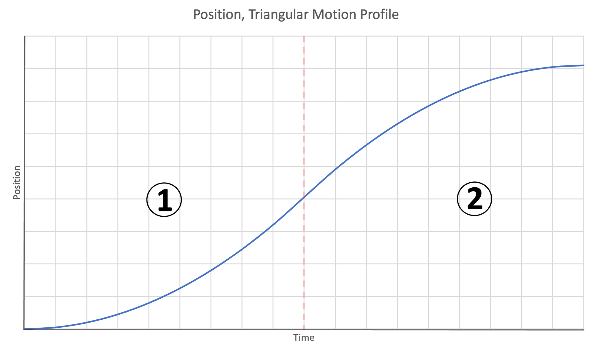
Figure 8: Motion profiles for triangular motion | Left- Acceleration | Center- Velocity | Right- Position
Like the trapezoidal motion profile, time/distance for the accelerating stages (1 and 2) are the same. The time required to complete the motion is twice the time to complete the first stage:
$$t_T = 2t_1\:[11]$$
Because the motion is triangular, the distance covered during stage 1 is half the total distance $x_1 = \frac{x_T}{2}$. The time to complete stage 1 is given by:
$$t_1 = \sqrt{\frac{\Delta x_T}{a}}\:[12]$$
Proof of Time for Acceleration Constrained Triangular Motion, Stage 1 (F)
For stage 1 of the trapezoidal motion profile, $v_{i} = 0$, $a = a$, and the travel distance is half the total travel distance $\Delta x = \frac{\Delta x_T}{2}$. We do not know $v_f$ because the target velocity is never reached. Substituting the stage 1 parameters into the second kinematic equation $[2]$, we obtain:
$$\Delta x = v_it + \frac{1}{2}at^2 \:[2]$$
$$\downarrow $$
$$\frac{\Delta x_T}{2} = 0 t_1+ \frac{1}{2}at_1^2$$
$$\downarrow $$
$$\Delta x_T= at_1^2$$
$$\downarrow $$
$$t_1 = \sqrt{\frac{\Delta x_T}{a}}$$
Substituting equation $[12]$ into $[11]$ yields the total time:
$$t_T = 2t_1\:[11]$$
$$\downarrow$$
$$t_T = 2\sqrt{\frac{\Delta x_T}{a}}$$
The condition for acceleration constrained motion is given by:
$$\Delta x_T < \frac{v_t^2}{a}$$
Proof of Condition for Acceleration Constrained Triangular Motion (G)
Recall from earlier equation $[12]$ which describes the time required to complete stage 1 of a triangular motion profile.
$$t_1 = \sqrt{\frac{\Delta x_T}{a}}\:[12]$$
Also recall equation $[4]$, which describes the relationship between final velocity, acceleration, and time for a constant acceleration segment with zero initial velocity:
$$t = \frac{v_f}{a}\: [4]$$
Substituting equation $[12]$ into $[4]$
$$\sqrt{\frac{\Delta x_T}{a}} = \frac{v_f}{a} $$
$$\downarrow$$
$$v_f = a\sqrt{\frac{\Delta x_T}{a}} $$
$$\downarrow$$
$$v_f = \sqrt{a\Delta x_T}\:[G1]$$
This is the final velocity of a triangular motion profile for a given acceleration and travel distance. If the motion profile is acceleration constrained, the target velocity is greater than the achievable final velocity, $v_t > v_f$. We can substitute $[G1]$ into the condition:
$$v_t > \sqrt{a\Delta x_T}$$
$$\downarrow$$
$$\frac{v_t^2}{a} > \Delta x_T$$
$$\downarrow$$
$$ \Delta x_T < \frac{v_t^2}{a}$$
Full Bang Bang Motion Solution
We've now demonstrated that we can solve for the time $t_T$ for any given combination of travel distance $\Delta x_T$, acceleration $a$, and target velocity $v_t$ (even target velocities that cannot be reached for certain distance/acceleration combinations). Depending on the choice of parameters, the profile will be either trapezoidal or triangular. We can condense these cases into a single equation that will return the motion time for any set of parameters:
$$\boxed{t_T = \begin{cases} \frac{\Delta x_T}{v_t} + \frac{v_t}{a} \text{ if } \Delta x_T \ge \frac{v_t^2}{a} \\ 2\sqrt{\frac{\Delta x_T}{a}} \text{ if } \Delta x_T < \frac{v_t^2}{a} \end{cases}}$$
Practical Example
Suppose our motion distance is $25mm$ and we fix the acceleration to $2000 \frac{mm}{s^2}$. Substituting into our bang bang motion time equation, we obtain:
$$t_T = \begin{cases} \frac{\Delta x_T}{v_t} + \frac{v_t}{a} \text{ if } \Delta x_T \ge \frac{v_t^2}{a} \\ 2\sqrt{\frac{\Delta x_T}{a}} \text{ if } \Delta x_T < \frac{v_t^2}{a} \end{cases}$$
$$\downarrow $$
$$t_T = \begin{cases} \frac{25}{v_t} + \frac{v_t}{2000} \text{ if } 25 \ge \frac{v_t^2}{2000} \\ 2\sqrt{\frac{25}{2000}} \text{ if } \Delta x_T < \frac{v_t^2}{2000} \end{cases}$$
We can simplify and rearrange the conditions:
$$t_T = \begin{cases} \frac{25}{v_t} + \frac{v_t}{2000} \text{ if } v_t \le 223.6 \\ 0.223 \text{ if } v_t > 223.6 \end{cases}$$
We can generate a plot of velocity vs time for this motion.
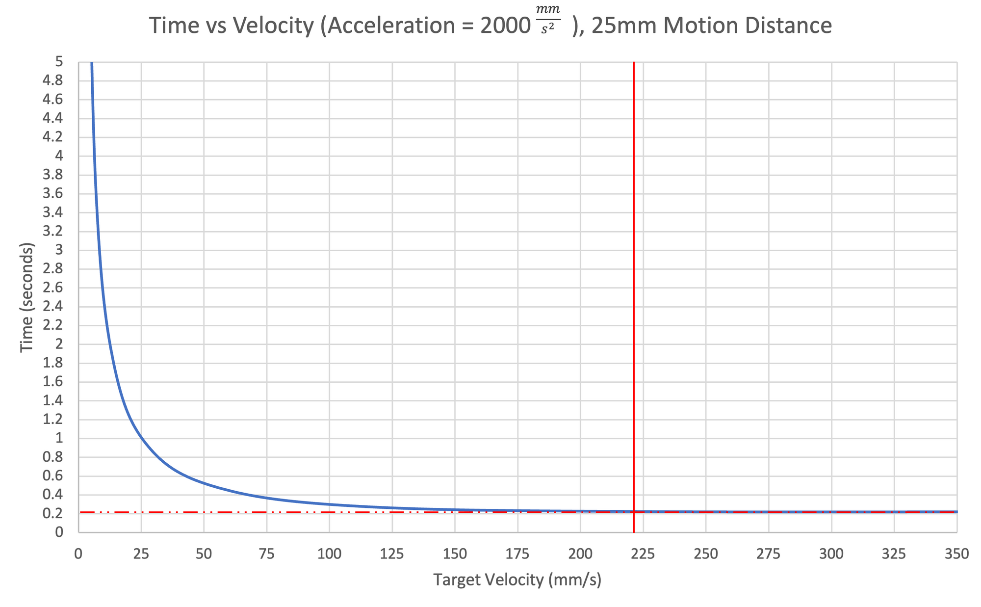
When the velocity is low, the time is high, and as the velocity increases, the time decreases until it converges to the time corresponding to the triangular motion profile. After this, there are no further time improvements because the motion is acceleration constrained.
This type of plot is just one example of this equation's usefulness. A robot's acceleration and velocity capabilities both require power. Suppose we are interested in designing a robot with a reasonable choice of velocity capability such that we balance the time to complete the motion with the power requirements of the robot.
Per Figure 9, a target velocity of $10\frac{mm}{s}$ would take $2.5s$, $50\frac{mm}{s}$ would take $0.53s$, and $220\frac{mm}{s}$ would take $0.22s$. We can make the following assessments:
- The $5x$ increase in speed $(10\frac{mm}{s} \rightarrow 50\frac{mm}{s})$ resulting in the move taking $21\%$ the time $(2.5s \rightarrow 0.53s)$ seems well justified.
- The $4.4x$ increase in speed $(50\frac{mm}{s} \rightarrow 220\frac{mm}{s})$ resulting in the move taking $42\%$ the time $(0.53s \rightarrow 0.22s)$ seems like a comparatively poor tradeoff.
These are the sort of decisions an engineer makes while designing a robot. Though this example may seem a little hand wavy, there are more rigid methods of making these decisions using optimization techniques. These will be covered in a future article.