Parametric Equations

Prerequisites- Basic Mathematics, Standard Vectors
Traditional functions of the form $y = f(x)$ accept an input $x$ and return an output $y$. When these functions are graphed, we put the input $x$ along the horizontal axis and the output $y$ along the vertical axis.
Consider the function $y = x^2$. The graph of this function is shown below:
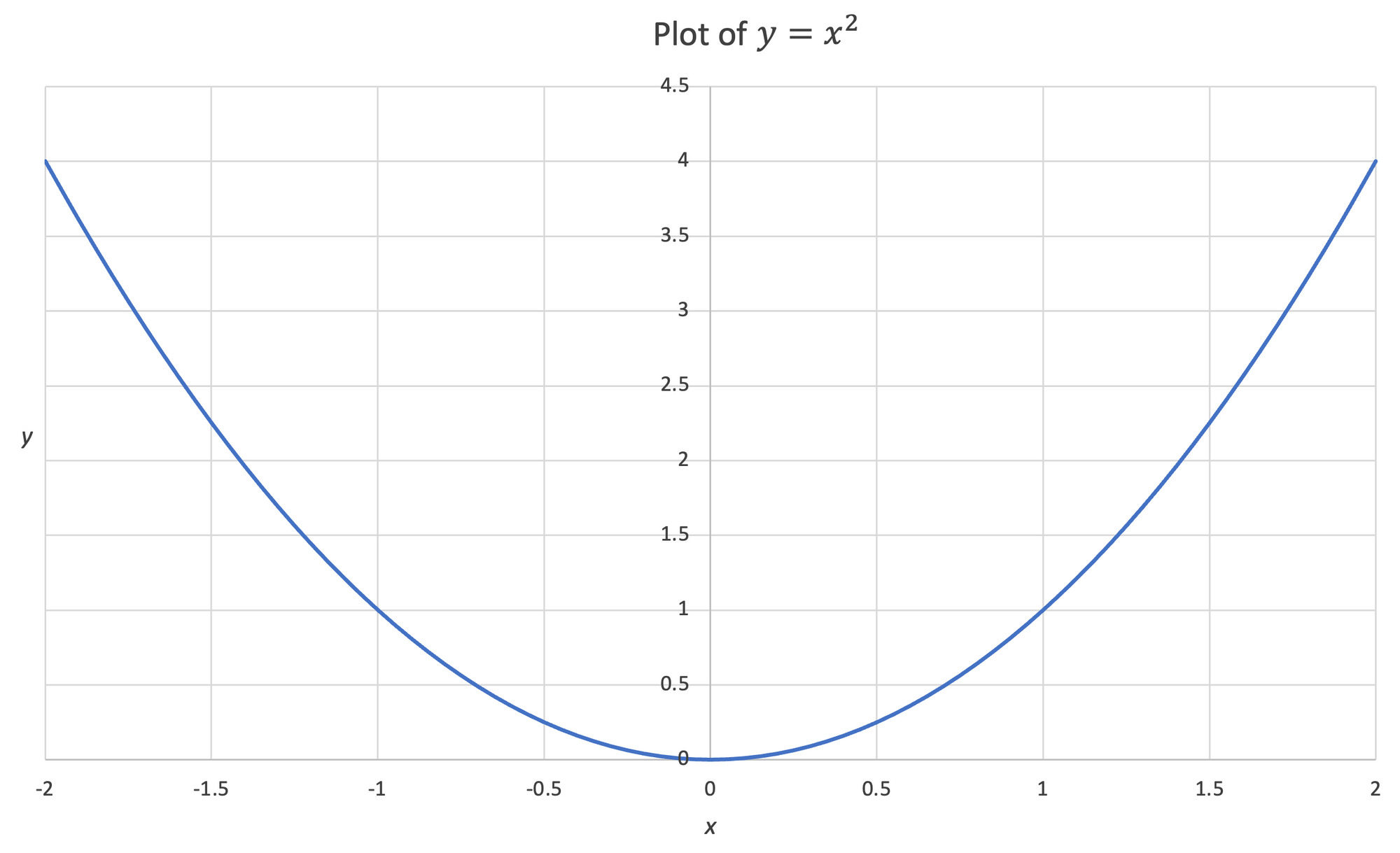
Functions are often quite aesthetic, they form all kinds of interesting shapes.
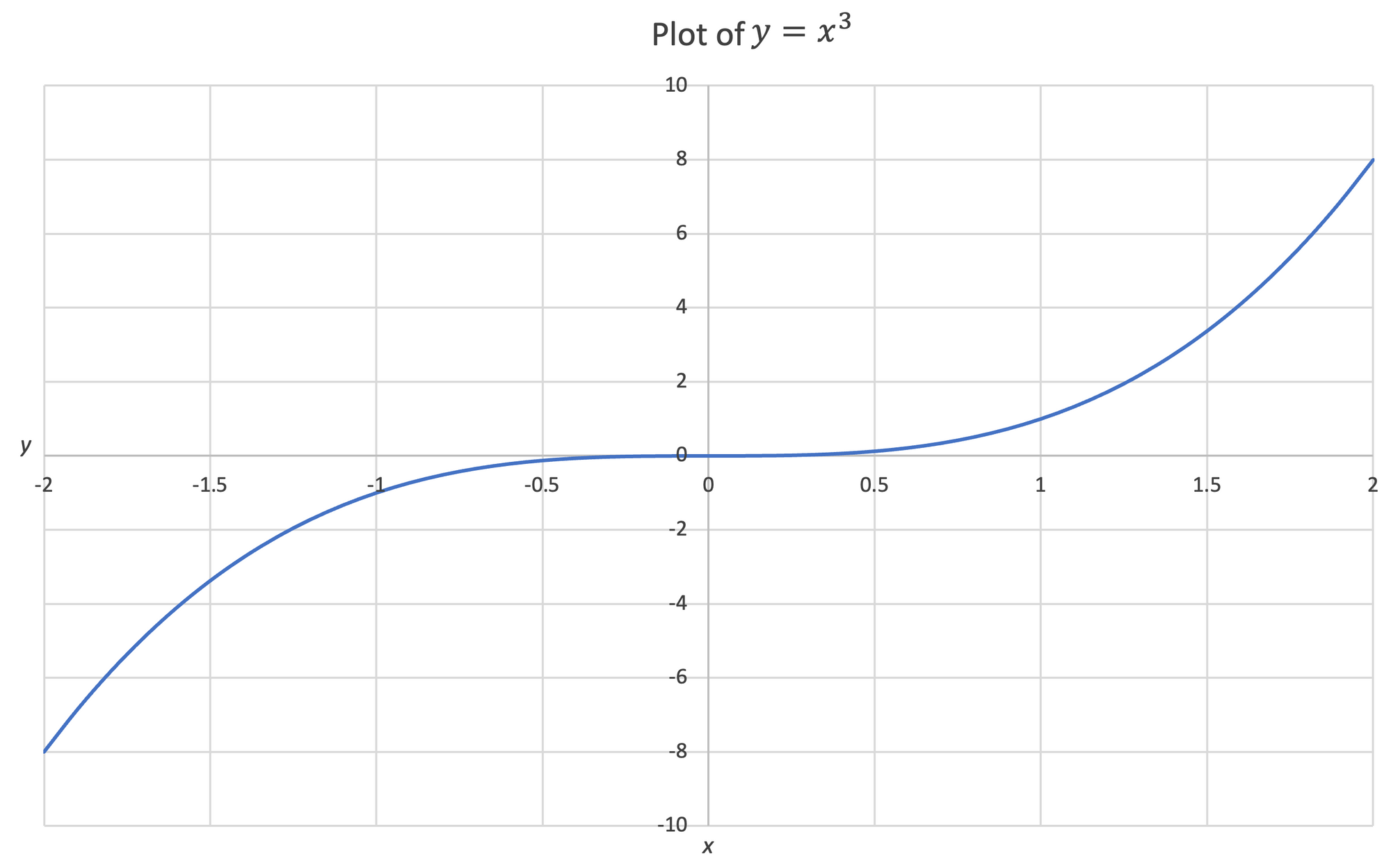
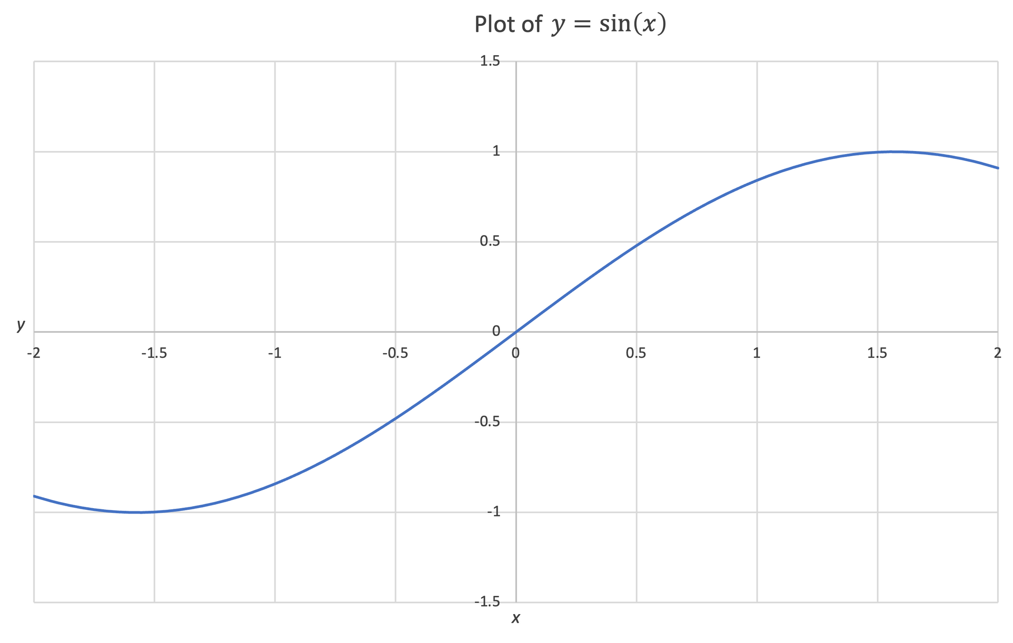
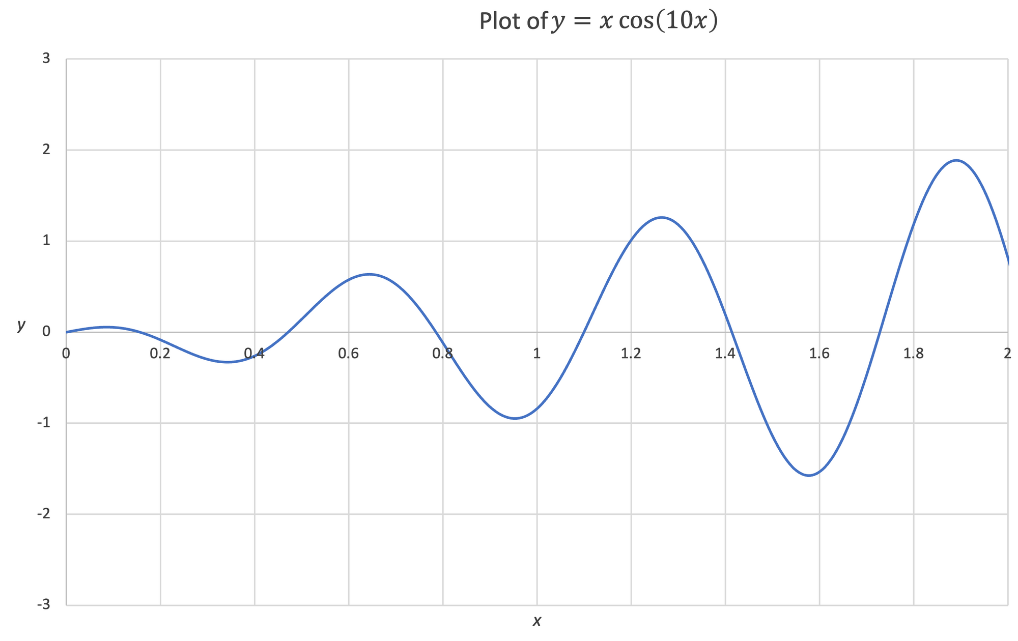
Figure 2:Left- Plot of the function $y = x^3$ | Center- Plot of the function $y = sin(x)$ | Right- Plot of the function $y = xcos(10x)$
Sometimes we desire to use functions to represent curves and paths. There are many reasons we might want to do this; architecture, motion graphics, roller coasters, civil planning, illustration, and mechanical engineering are just a few examples.


Figure 3:Upper Left- Photo of Zentrum Paul Klee, by Ricardo Gomez, courtesy of unsplash | Upper Center- Electrical path animation by motionstock, courtesy of pixabay | Upper Right- Three dimensional curves are used to design roller coasters, photo by Mateo Fernandez, courtesy of unsplash | Lower Left- Curves are used to plan roads, photo by David Talley, courtesy of unsplash | Lower Center- Digital illustrations can be created using curves, by cromaconceptovisual, courtesy of pixabay | Lower Right- Curves are used extensively in mechanical engineering design, by PIRO4D, courtesy of pixabay
I don't think I can overstate how important curves are. Though the value of using math to draw curves is not often emphasized in math courses, very few of our modern advancements would be possible without them.
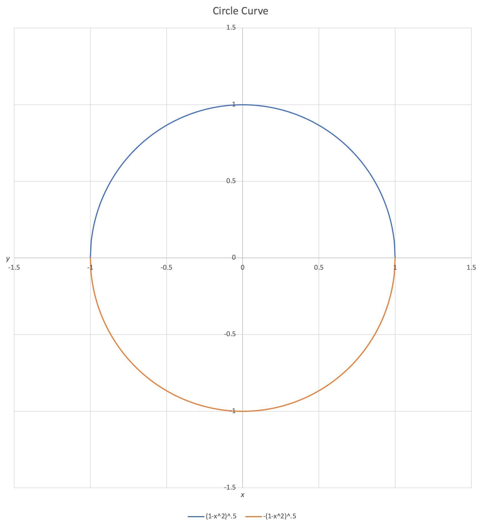
One means of creating curves from traditional functions $y = f(x)$ is to stitch together multiple functions to draw a shape. The below equation creates a circle by stitching together two semicircles:
$$y = \begin{cases} \sqrt{1-x^2} \\ -\sqrt{1-x^2}\end{cases},\: -1 \le x \le 1$$
If we plot this equation, we obtain the below curve:
Stitching makes it possible to draw many kinds of curves, but there is an unfortunate difficulty involved. For each function, each input $x$ corresponds to just one output $y$. This makes it challenging to draw certain curves. Any curve that reverses in $x$ must be represented by a stitched function broken up where the tangent is vertical.
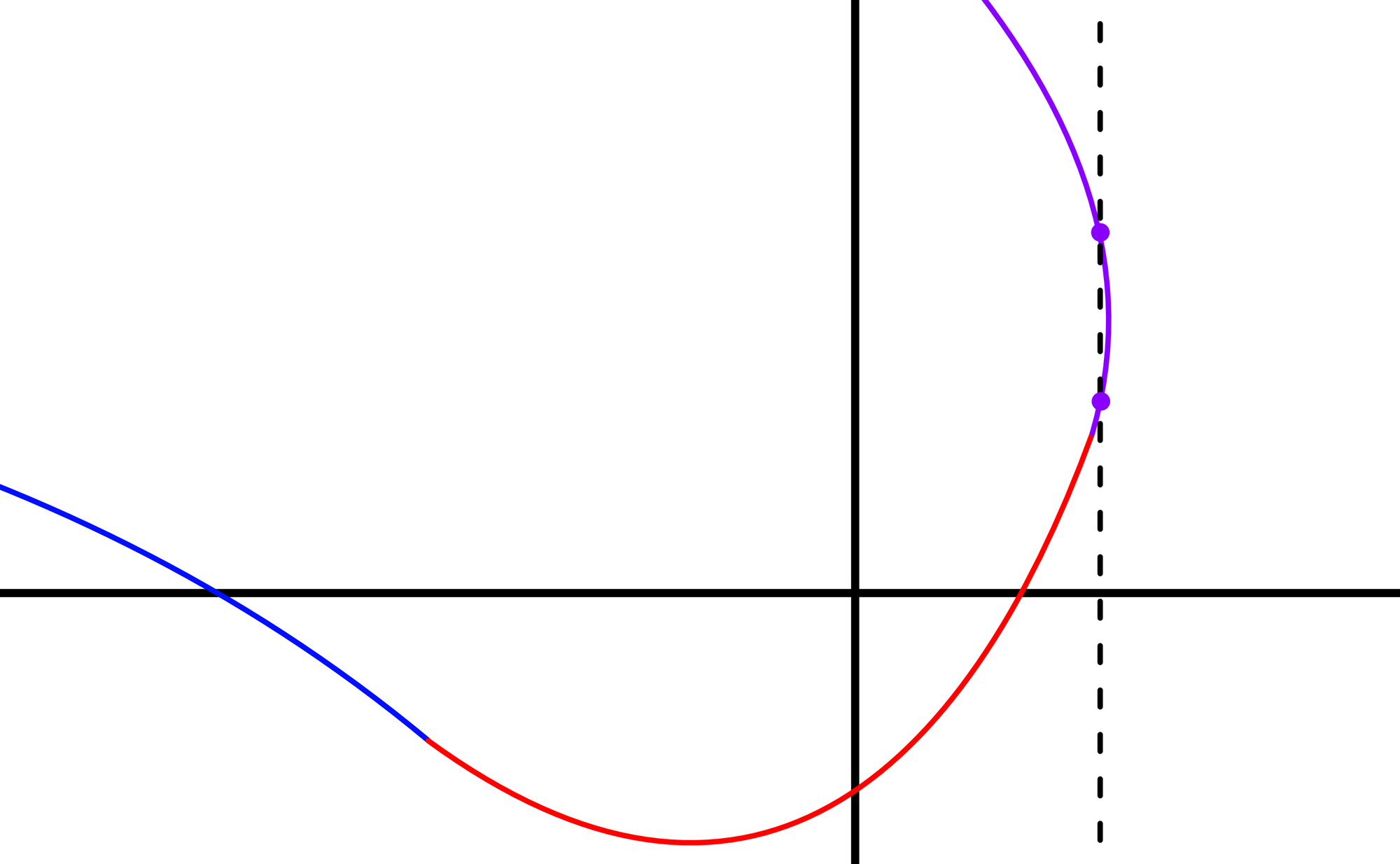
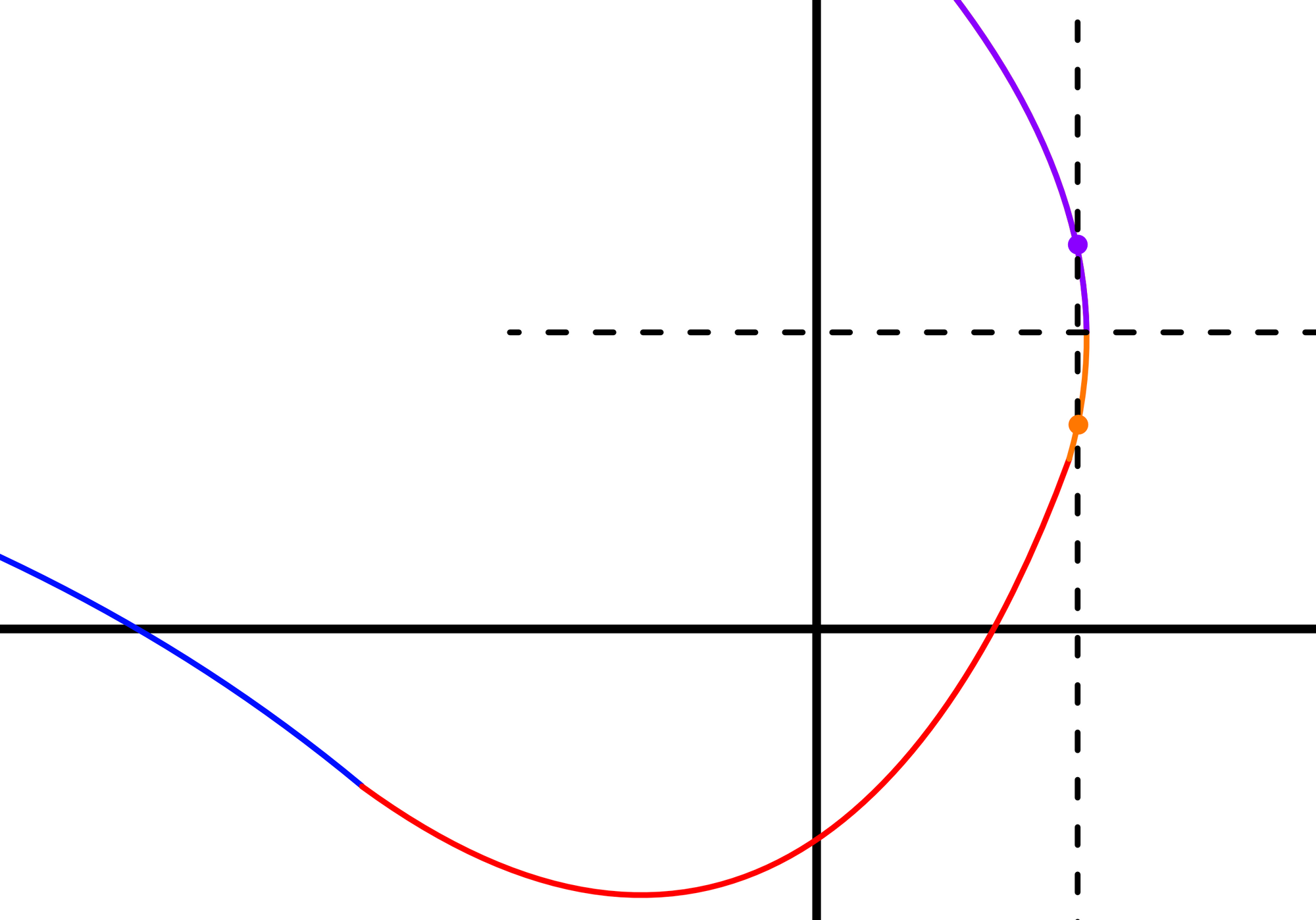
Figure 5: A chain of functions is being used to draw an interesting curve. | Left- This chain is invalid because the purple function has multiple $y$ values for some $x$ values | Right- This chain is valid. Each function contains only one output $y$ for each input $x$.
This is all rather complicated. Instead of representing paths as stitched functions $y = f(x)$, an alternative would be to introduce a new variable $s$ and define both $x$ and $y$ as functions of $s$:
$$x = f(s),\: y = g(s)$$
This is called a parametric equation. Some educational resources choose to use the letter $t$ to represent the parameter rather than $s$ but because $t$ is often associated with time, I prefer $s$.
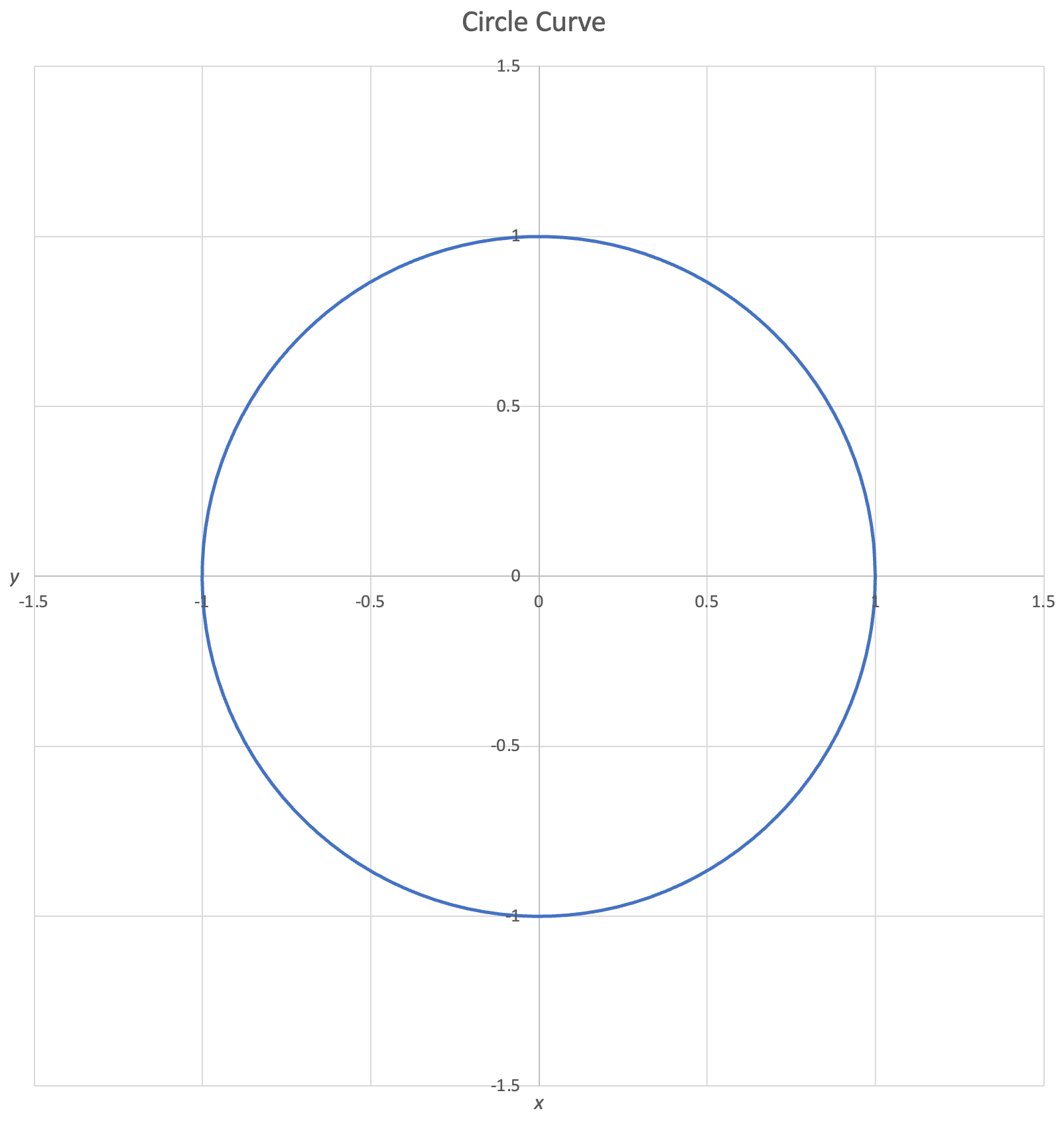
If we wanted to represent a circle using a parametric equation, we could use the below function:
$$x = cos(s),\: y = sin(s)$$
For this equation, a plot of $y$ vs $x$ is shown below:
Remember, $x$ and $y$ are independent functions of $s$. It is possible to also graph each coordinate's function with respect to $s$, $x(s)$ and $y(s)$.
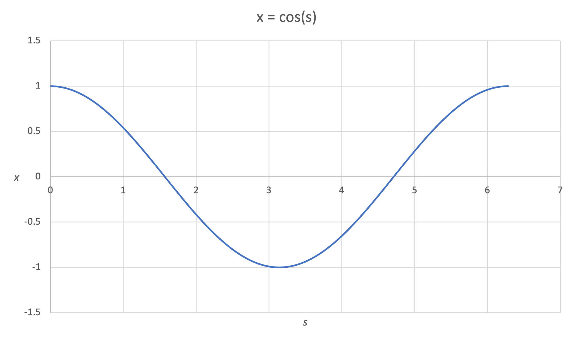
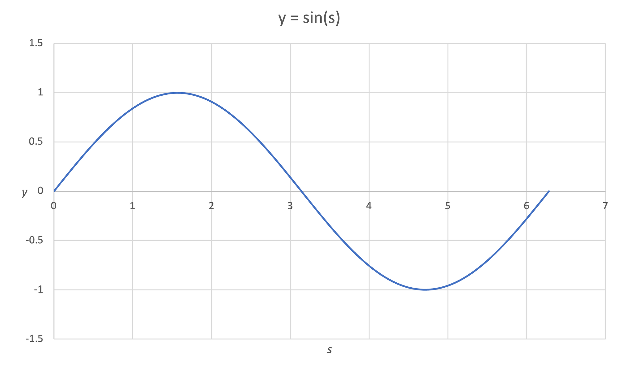
Figure 7: The functions corresponding to both the $x$ coordinate $x(s)$ (shown on left) and $y$ coordinate $y(s)$ (shown on right) can be plotted independently.
Though we call them equations, these are all functions. They accept an input $s$ and return outputs $x$ and $y$.
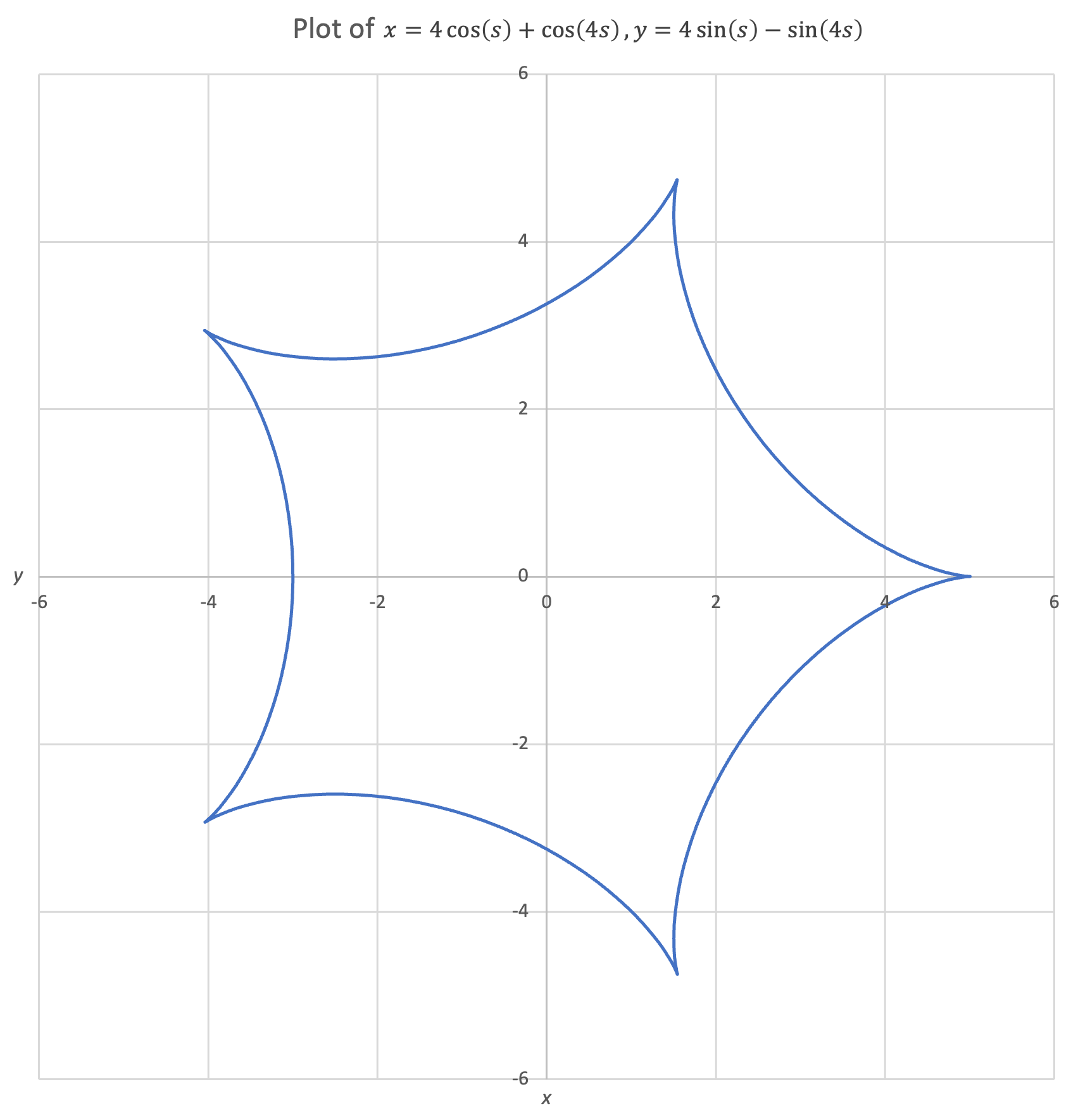
Another parametric equation yields a sort of star path:
$$x(s) = 4 cos(s) + cos(4s),\:y(s) = 4 sin(s) - sin(4s)$$
Vector Representation of Parametric Functions
To simplify their notation, parametric functions are often represented as vectors. $\overline{p}(s)$ represents the coordinates of the parametric function with parameter $s$:
$$\overline{p}(s) = \begin{bmatrix} x(s) \\ y(s) \end{bmatrix}$$
For our earlier parametric equation corresponding to a circle, we would write the vector form of the parametric equation as:
$$\overline{p}(s) = \begin{bmatrix} cos(s) \\ sin(s) \end{bmatrix}$$
Time Based Parametric Equations
Up to this point, all of the curves we have been working with have been functions of parameter $s$ and we have used these functions to draw all sorts of interesting shapes. We normally evaluate these kinds of functions at many different values of $s$ to obtain the overall shape. The below example in Microsoft Excel demonstrates this process.
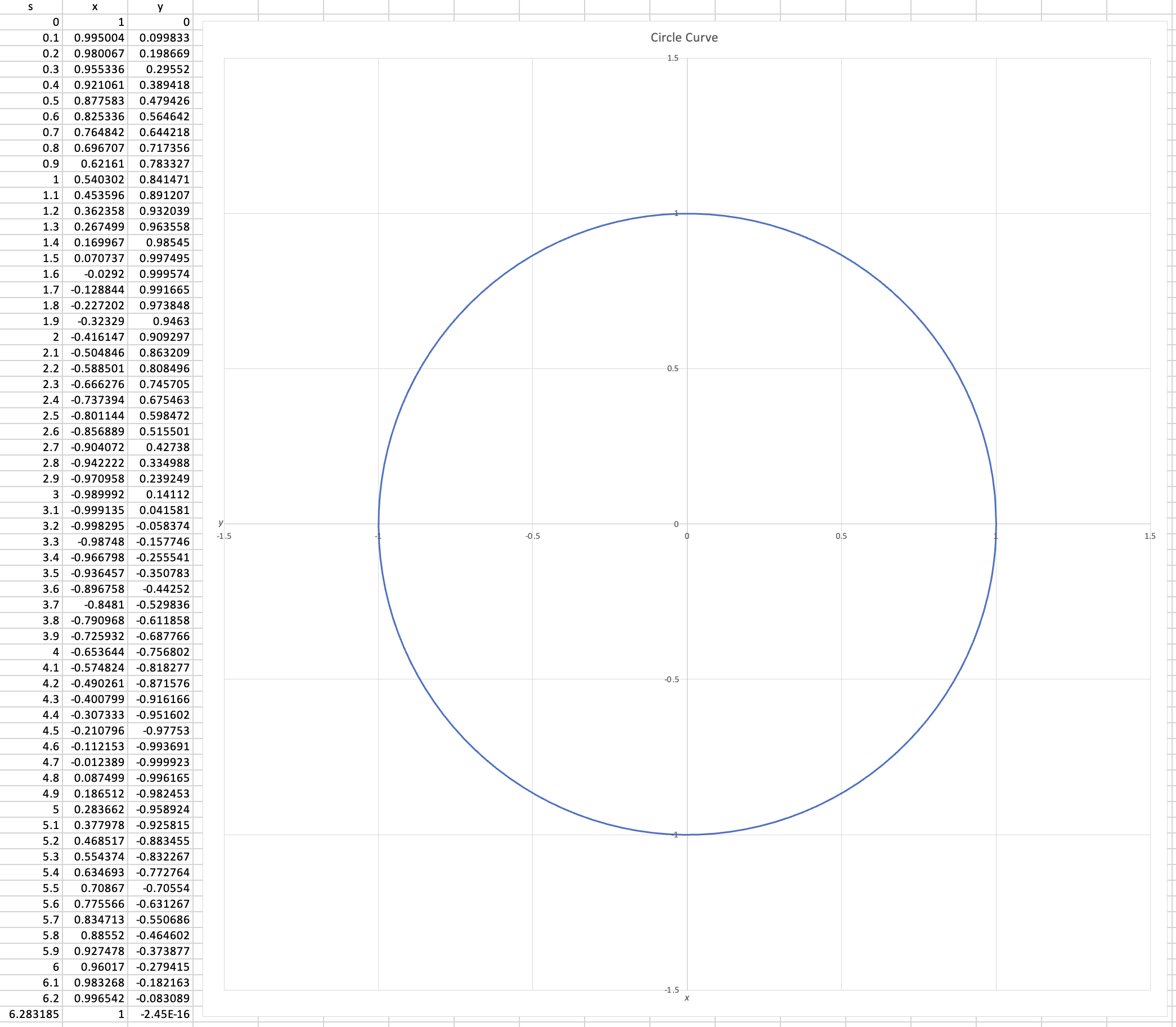
Instead of drawing a shape, we are sometimes interested in using parametric equations to represent how an object changes with time. We do this by assigning a property of the object ($x$ postion, $y$ position, size, rotation, etc) to the parametric equation. For example, we can represent a point moving in a circle by assigning its $x$ and $y$ positions to the circle parametric equation example and using $t$ (time) as the parameter instead of $s$:
$$\overline{p}(t) = \begin{bmatrix} cos(t) \\ sin(t) \end{bmatrix}$$
Figure 10: Animation demonstrating the time evolution of a point whose position is given by the parametric equation $\overline{p}(t) = \begin{bmatrix} cos(t) \\ sin(t) \end{bmatrix}$.
Three Dimensional Parametric Equations
If we wanted to add another dimension to our parametric equation and draw a curve in three dimensions, we simply add a function for the $z$-axis to our equation:
$$x = f(s),\:y = g(s),\:z = h(s)$$
This also has a vector representation:
$$\overline{p}(s) = \begin{bmatrix} f(s) \\ g(s) \\ h(s) \end{bmatrix}$$
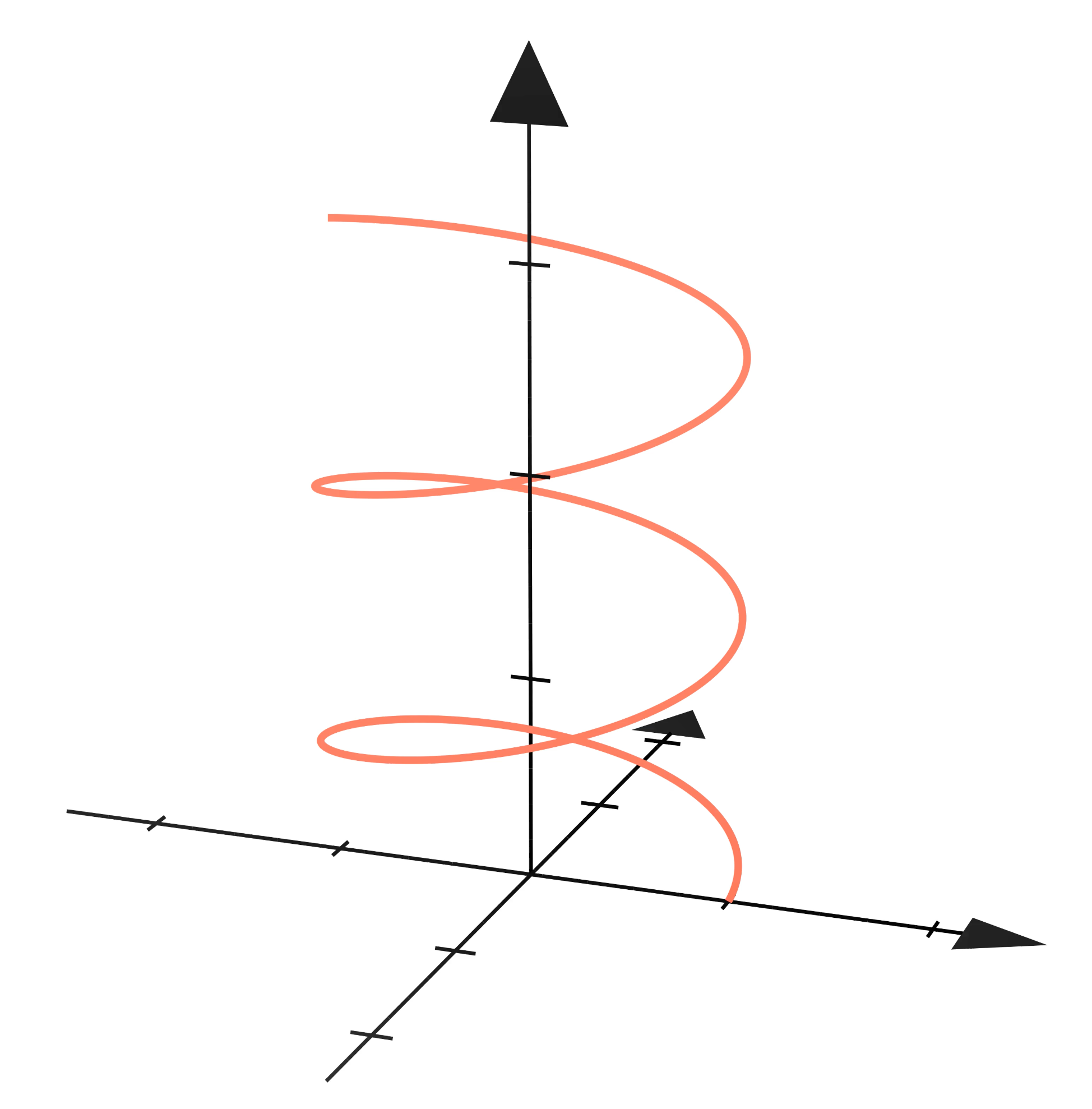
One common example of a three dimensional parametric equation is a helix:
$$\overline{p}(s) = \begin{bmatrix} cos(s) \\ sin(s) \\ \frac{s}{5} \end{bmatrix}$$
Four+ Dimensional Parametric Equations
Drawing a path in three dimensions instead of two dimensions was very straightforward. The method of extending 2D to 3D can be applied to draw a path through any number of dimensions.
One example of a higher dimensional path is to describe the $x$, $y$, $z$ and $\theta$ coordinates of an object with respect to time, where $\theta$ is the absolute angle with respect to the $z$-axis (in degrees):
$$x = f(t),\:y = g(t),\:z = h(t),\:\theta = k(t)$$
We can use the helical parametric equation developed earlier and use it to describe the position and orientation of a cube:
$$\overline{p}(t) = \begin{bmatrix} cos(t) \\ sin(t) \\ \frac{t}{5} \\ 360t \end{bmatrix}$$
Figure 12: Animation demonstrating the time evolution of a cube whose position and rotation is given by the parametric equation $\overline{p}(t) = \begin{bmatrix} cos(t) \\ sin(t) \\ \frac{t}{5} \\ 360t \end{bmatrix}$.
These types of equations have a lot of potential applications.
One Dimensional Parametric Equations
A one dimensional curve has only one function:
$$x = f(s)$$
A plot of $x$ vs $s$ looks like a traditional function. The parametric plot of this curve looks like a number line and shows the overall bounds of $x$.
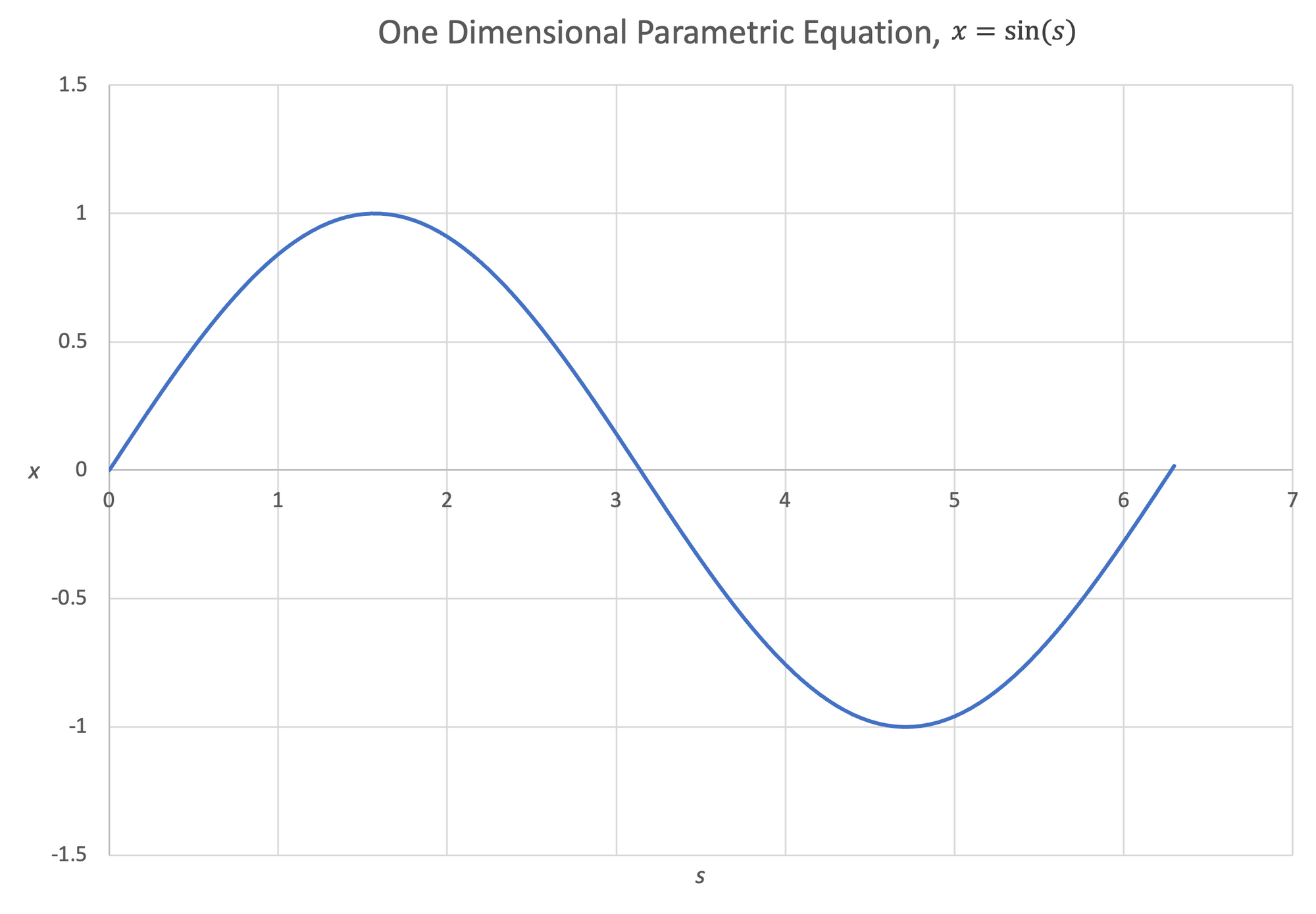
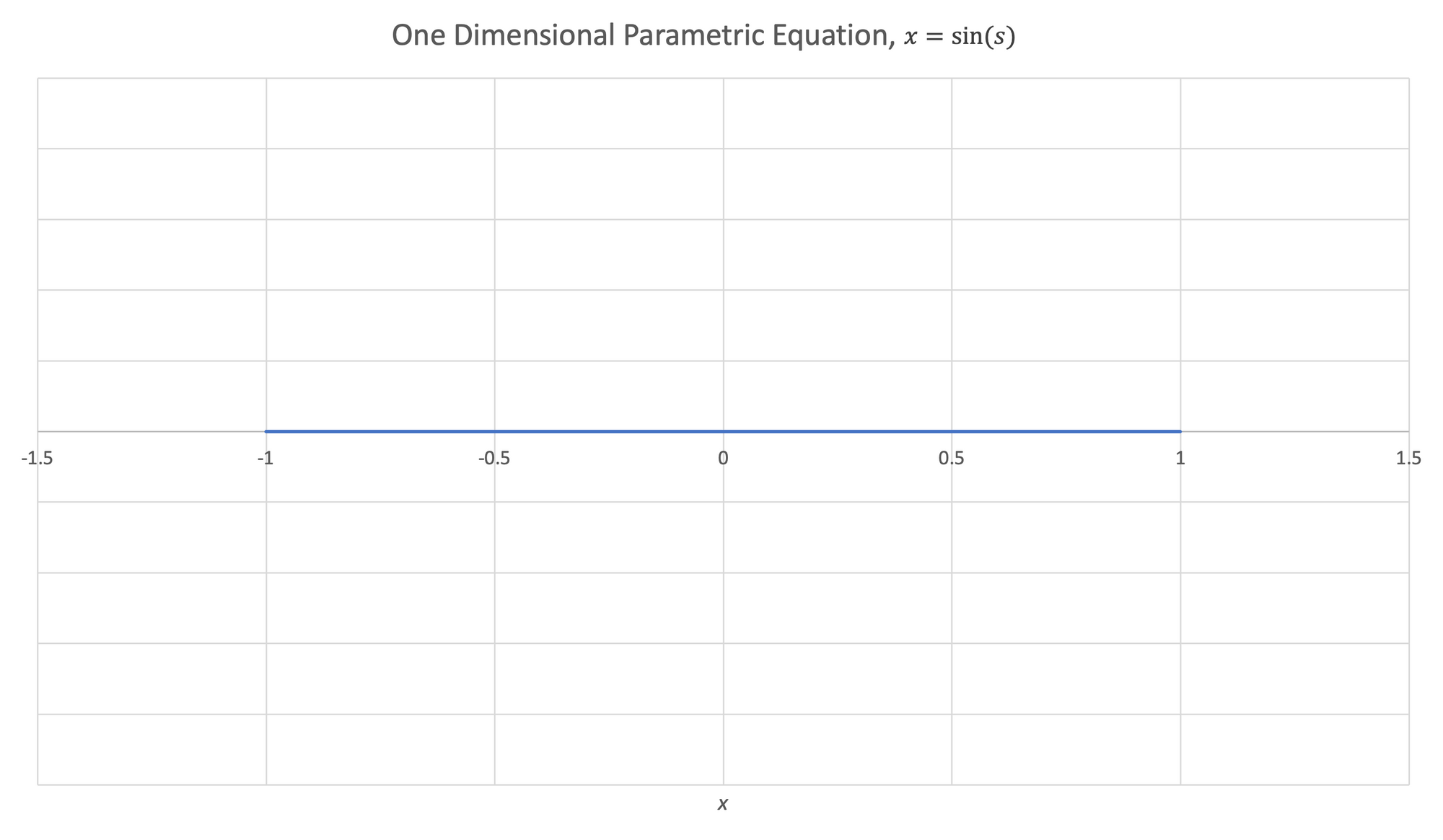
Figure 13:Left- Plot of $x$ vs $s$, $x = sin(s)$ | Right- Plot of parametric equation $x = sin(s)$
While a one dimensional parametric equations is mathematically valid, it has less utility than higher dimension parametric equations.
Polynomial Parametric Equations
Perhaps the most useful application of parametric equations is for generating smooth curves. These curves are typically generated using polynomial parametric equations. One example of a polynomial parametric equation is:
$$x = s^2+2s,\:y = s^3-s^2+4s$$
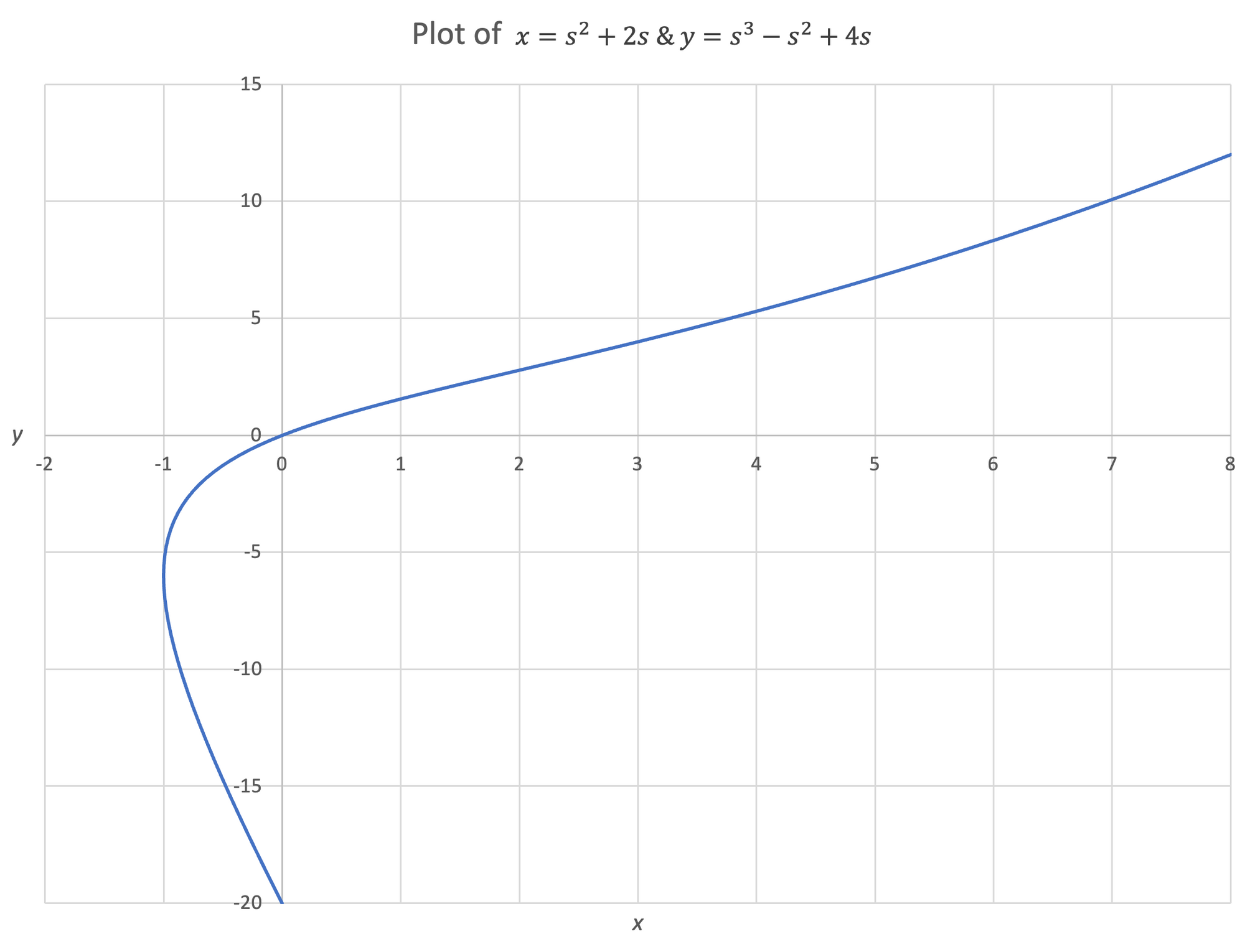
These curves have many different specific names (Bezier curves are extremely common) and we can connect curves together to make a longer curve called a spline. For simplicity, we will keep these curves as two dimensional but they can be easily extended into three or more dimensions.
Linear Polynomial Parametric Equations (1st Order)
The simplest polynomial function is a linear function $y = Ax + b$. The general linear parametric function is:
$$x(s) = As + B,\:y(s) = Cs + D$$
where $A$, $B$, $C$, and $D$ are numbers that shape the curve.
Quadratic Polynomial Parametric Equations (2nd Order)
Quadratic polynomial curves are based on the quadratic function $y = Ax^2 + Bx + C$. The general quadratic parametric function is:
$$x(s) = As^2 + Bs + C,\:y(s) = Ds^2 + Es + F$$
where $A$, $B$, $C$, $D$, $E$, and $F$ are numbers that shape the curve.
Cubic Polynomial Parametric Equations (3rd Order)
Cubic polynomial curves are based on the cubic function $y = Ax^3 + Bx^2 + Cx + D$
$$x(s) = As^3 + Bs^2 + Cs + D,\:y(s) = Es^3 + Fs^2 + Gs + H$$
where $A$, $B$, $C$, $D$, $E$, $F$, $G$, $H$ are numbers that shape the curve.
The prior example in figure 14, $x = s^2+2s,\:y = s^3-s^2+4s$, is a cubic polynomial parametric equation.
Nth Order Polynomial Parametric Equations
We've described 1st (Linear), 2nd (Quadratic), and 3rd (Cubic) order polynomial functions, there is nothing restricting the maximum order of polynomials. It is possible to create a hundredth order polynomial curve (though there would notably be $202$ curve shaping numbers ($101$ for each dimension) that need to be defined.
Derivatives of Parametric Equations
Like traditional functions, parametric equations are differentiable. Suppose we have a parametric function
$$x(s) = 4s^2 + 3s + 2,\:y(s) = 2s^2 - 4s + 4$$
1st Derivative $\frac{d}{ds}$
Taking the derivative of this function with respect to $s$ is very simple; we take the derivative of each part of the parametric function:
$$\frac{d}{ds}x(s) = \frac{d}{ds}(4s^2 + 3s + 2),\:\frac{d}{ds}y(s) = \frac{d}{ds}(2s^2 - 4s + 4)$$
$$\frac{d}{ds} x(s) = 8s + 3,\:\frac{d}{ds} y(s) = 4s - 4$$
We could have also used the vector form:
$$\overline{C}(s) = \begin{bmatrix} 4s^2 + 3s + 2 \\ 2s^2 - 4s + 4 \end{bmatrix}$$
$$\frac{d}{ds}\overline{C}(s) = \frac{d}{ds}\begin{bmatrix} 4s^2 + 3s + 2 \\ 2s^2 - 4s + 4 \end{bmatrix}$$
$$\frac{d}{ds} \overline{C}(s) = \begin{bmatrix} 8s + 3 \\ 4s - 4 \end{bmatrix}$$
This first derivative is the rate of change in each dimension with respect to the parameter $s$.
If we project a line outward from the curve along the direction of the first derivative, we observe that this is curve's tangent:
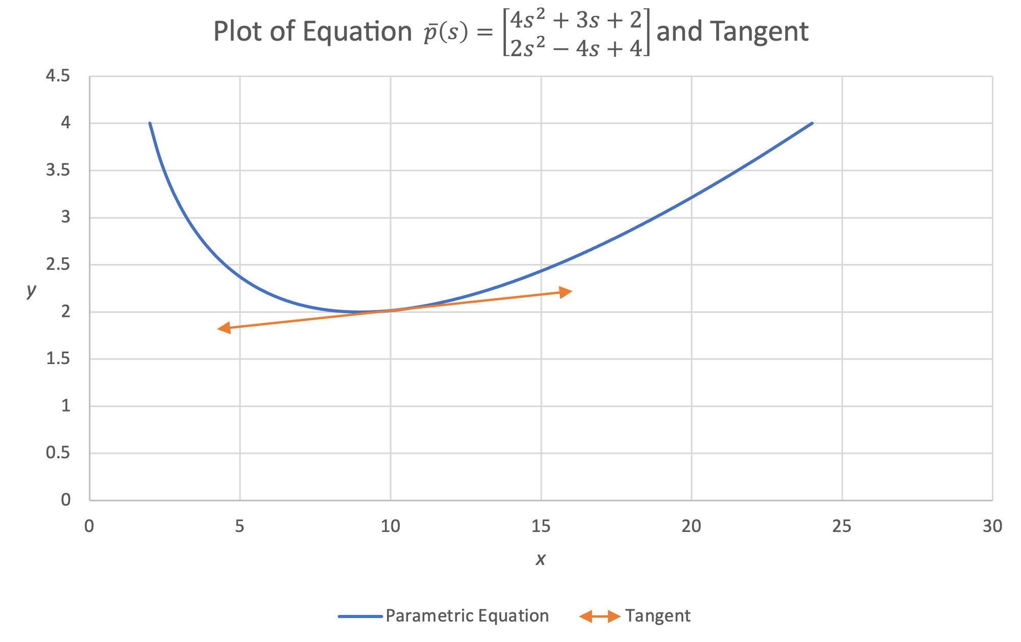
If we divide the y component of the derivative by the x component of the derivative, we can obtain the slope of the curve we associate with traditional functions:
$$\frac{dy}{dx} \overline{C}(s) = \frac{\frac{d}{ds}\overline{C}_y}{\frac{d}{ds}\overline{C}_x}$$
In the case of our example,
$$\frac{dy}{dx} C(s) = \frac{4s - 4}{8s + 3}$$
2nd Derivative $\frac{d^2}{ds^2}$
Taking the second derivative is similar to taking the 1st derivative. We just take the derivative twice:
$$\frac{d^2}{ds^2} \overline{C}(s) = \frac{d}{ds}\left(\frac{d}{ds} \overline{C}(s)\right)$$
In the case of our earlier example, we found:
$$\overline{C}(s) = \begin{bmatrix} 4s^2 + 3s + 2 \\ 2s^2 - 4s + 4 \end{bmatrix}$$
$$\frac{d}{ds} \overline{C}(s) = \begin{bmatrix} 8s + 3 \\ 4s - 4 \end{bmatrix}$$
$$\frac{d}{ds}\left(\frac{d}{ds} \overline{C}(s)\right) = \begin{bmatrix} 8 \\ 4 \end{bmatrix}$$
Similar to the 1st derivative, we can calculate the traditional 2nd derivative $\frac{d^2y}{dx^2}$:
$$\frac{d^2y}{dx^2} \overline{C}(s) = \frac{\frac{d^2}{ds^2}\overline{C}_y}{\frac{d^2}{ds^2}\overline{C}_x}$$
In our example, we find that
$$\frac{d^2y}{dx^2} = \frac{4}{8} = 0.5$$
Nth Order Derivatives
Taking higher order derivatives continues the general pattern:
$$\frac{d^n}{ds^n} \overline{C}(s) = \frac{d}{ds}\left(...\frac{d}{ds}\left(\frac{d}{ds}\left(\frac{d}{ds} \overline{C}(s)\right)\right)...\right)$$
We can also find any nth order derivative $\frac{d^ny}{dx^n}$:
$$\frac{d^ny}{dx^n} \overline{C}(s) = \frac{\frac{d^n}{ds^n}\overline{C}_y}{\frac{d^n}{ds^n}\overline{C}_x}$$
Anti-Derivatives (Indefinite Integrals)
Anti-derivatives (also sometimes called indefinite integrals) are simply the inverse of derivatives. Like derivatives, anti-derivatives are applied to each component of the parametric function.
$$\overline{C}(s) = \int \left( \frac{d}{ds} \overline{C}(s) \right)$$
Importantly, similar to the anti-derivatives of traditional functions, this process introduces a set of integration constant terms $c_x, c_y,...$. We need to define these constant terms in order to obtain the original path.
Example
$$\frac{d}{ds} \overline{C}(s) = \begin{bmatrix} 8s+ 3 \\ 4s - 4 \end{bmatrix}$$
$$\int \left(\frac{d}{ds} \overline{C}(s) \right) = \int \begin{bmatrix} 8s + 3 \\ 4s - 4 \end{bmatrix}$$
$$\int \left(\frac{d}{ds} \overline{C}(s) \right) = \begin{bmatrix} 4s^2 + 3s + c_x \\ 2s^2 - 4s + c_y \end{bmatrix}$$
In order to obtain our original parametric function, we would have to know it and observe the values for the constants:
$$x(s) = 4s^2 + 3s + 2,\:y(s) = 2s^2 - 4s + 4$$
Therefore, $c_x = 2$ and $c_y = 4$.
In the absence of any information on the constants, it is common to assign them equal to zero. In this case, it is important to recognize that $\int \left(\frac{d}{ds} \overline{C}(s) \right) \ne \overline{C}(s)$ because we are missing the value for the constants.
Tangent Direction of Parametric Functions
It can be very useful to know the direction a parametric function is pointing in for a given $s$. This is given by the unit vector of the derivative, which is found by dividing the derivative by the magnitude of itself:
$$\hat{u}_{Ct} = \frac{\frac{d}{ds}\overline{C}(s)}{||\frac{d}{ds}\overline{C}(s)||}$$
Using the identity:
$$\overline{A} \cdot \overline{A} = ||\overline{A}||^2$$
we can obtain the equation for the tangent direction:
$$\hat{u}_{Ct} = \frac{\frac{d}{ds}\overline{C}(s)}{\left(\frac{d}{ds}\overline{C}(s) \cdot \frac{d}{ds}\overline{C}(s)\right)^{0.5}}$$
Example
In the case of our example:
$$\overline{C}(s) = \begin{bmatrix} 4s^2 + 3s + 2 \\ 2s^2 - 4s + 4 \end{bmatrix}$$
$$\frac{d}{ds} \overline{C}(s) = \begin{bmatrix} 8s + 3 \\ 4s - 4 \end{bmatrix}$$
Substituting into our direction equation, we obtain:
$$\hat{u}_{Ct} = \frac{\begin{bmatrix} 8s + 3 \\ 4s - 4 \end{bmatrix}}{\left(\begin{bmatrix} 8s + 3 \\ 4s - 4 \end{bmatrix} \cdot \begin{bmatrix} 8s + 3 \\ 4s - 4 \end{bmatrix}\right)^{0.5}}$$
$$\hat{u}_{Ct} = \frac{\begin{bmatrix} 8s + 3 \\ 4s - 4 \end{bmatrix}}{\left((8s + 3)(8s + 3) + (4s-4)(4s-4)\right)^{0.5}}$$
$$\hat{u}_{Ct} = \frac{\begin{bmatrix} 8s + 3 \\ 4s - 4 \end{bmatrix}}{\left((64s^2 + 48s + 9)+ (16s^2 -32s + 16)\right)^{0.5}}$$
$$\hat{u}_{Ct} = \frac{\begin{bmatrix} 8s + 3 \\ 4s - 4 \end{bmatrix}}{\left(80s^2 + 16s + 25\right)^{0.5}}$$
$$\hat{u}_{Ct} = \frac{1}{\left(80s^2 + 16s + 25\right)^{0.5}}\begin{bmatrix} 8s + 3 \\ 4s - 4 \end{bmatrix}$$
