Jan 21, 2024 8 min read

Standard Vectors

Prerequisites Required- Trigonometric Functions

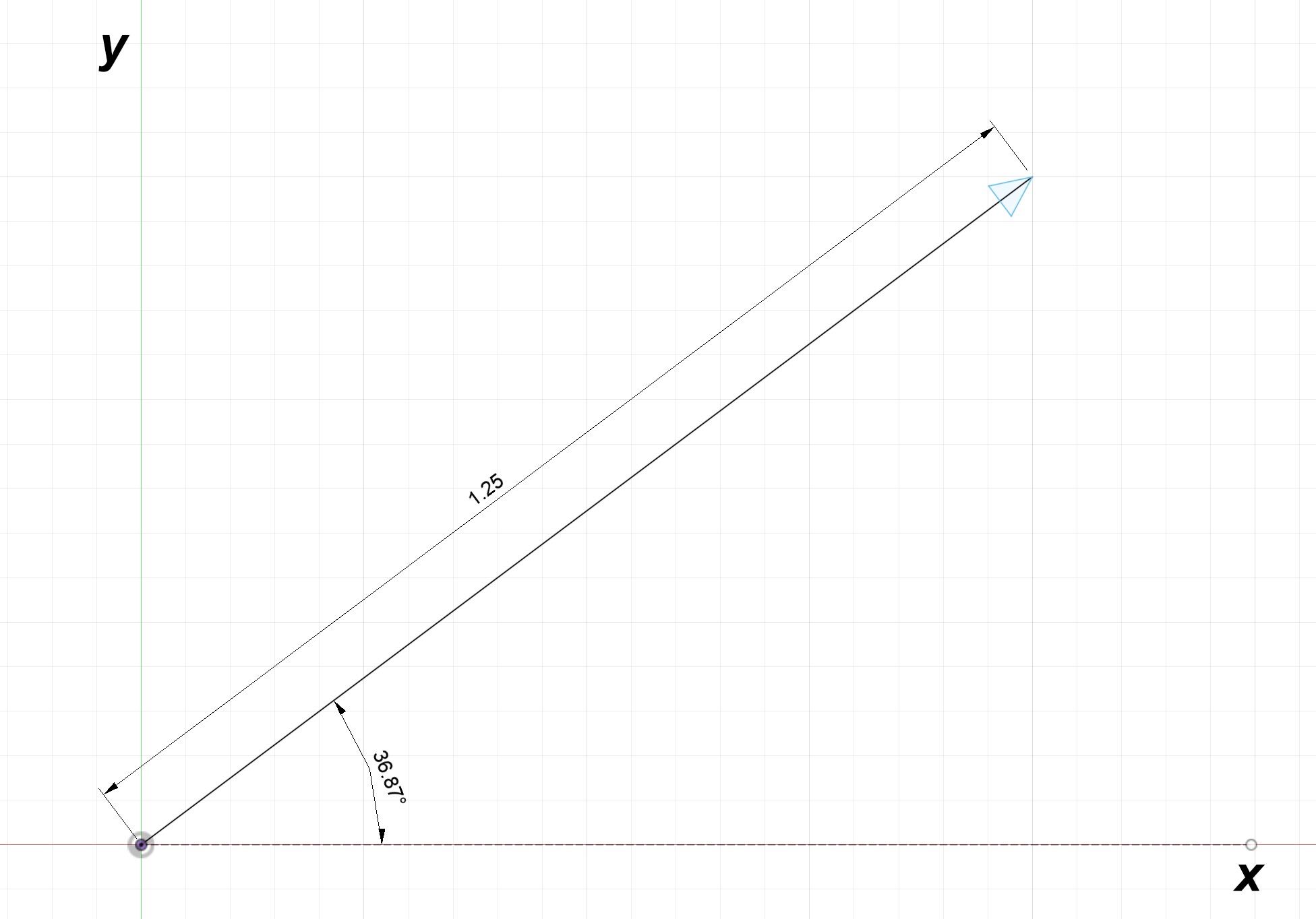
Throughout physics and engineering, few mathematical concepts are as pervasive as vectors. A vector is a mathematical representation for something with both direction and magnitude. One example of a vector is a point to point line, shown in the diagram below; it has both a length and a direction.

Vectors are not strictly limited to representing lines; they can be used to describe any quantity with direction and magnitude (distance, velocity, acceleration, force, etc.).

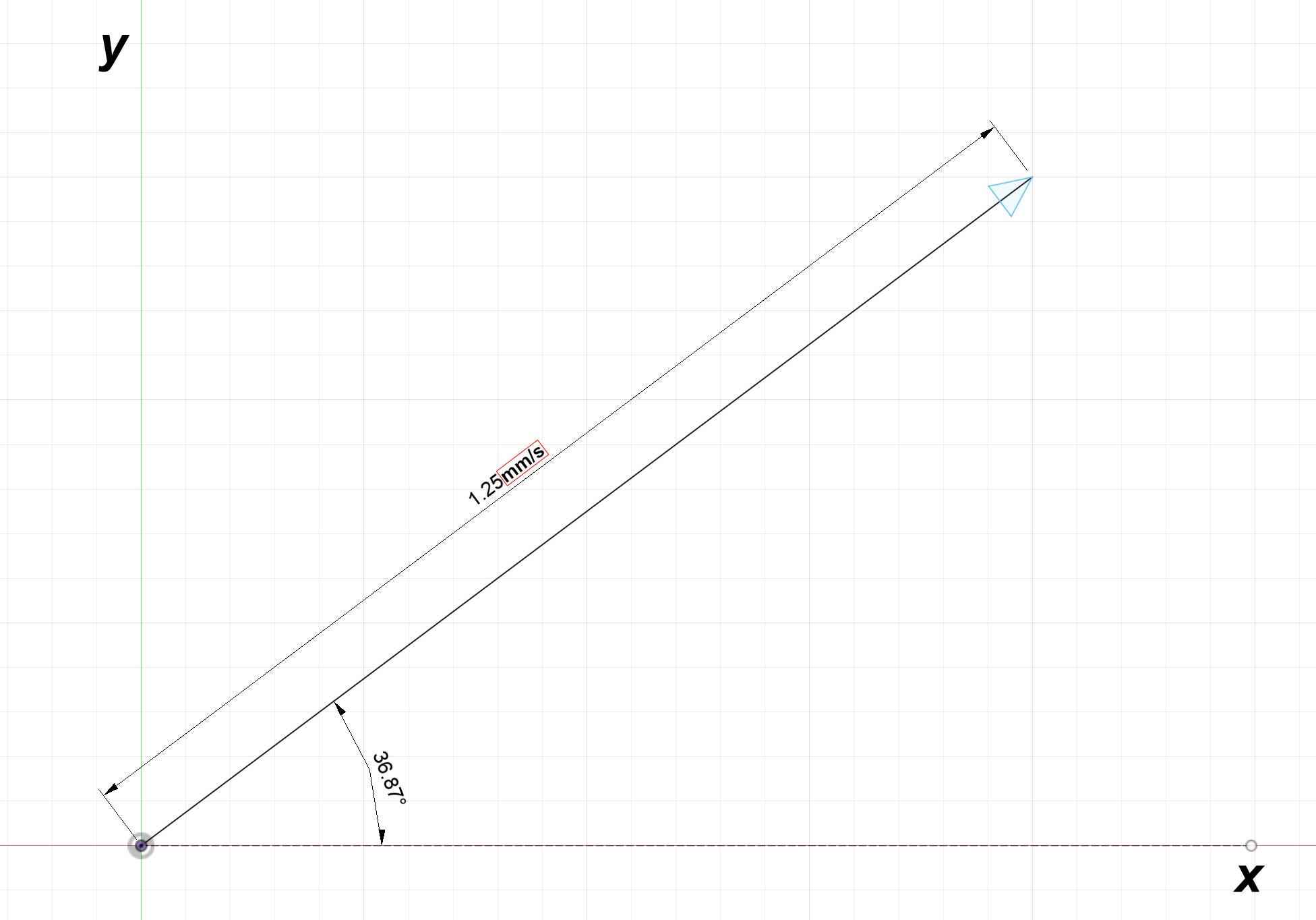
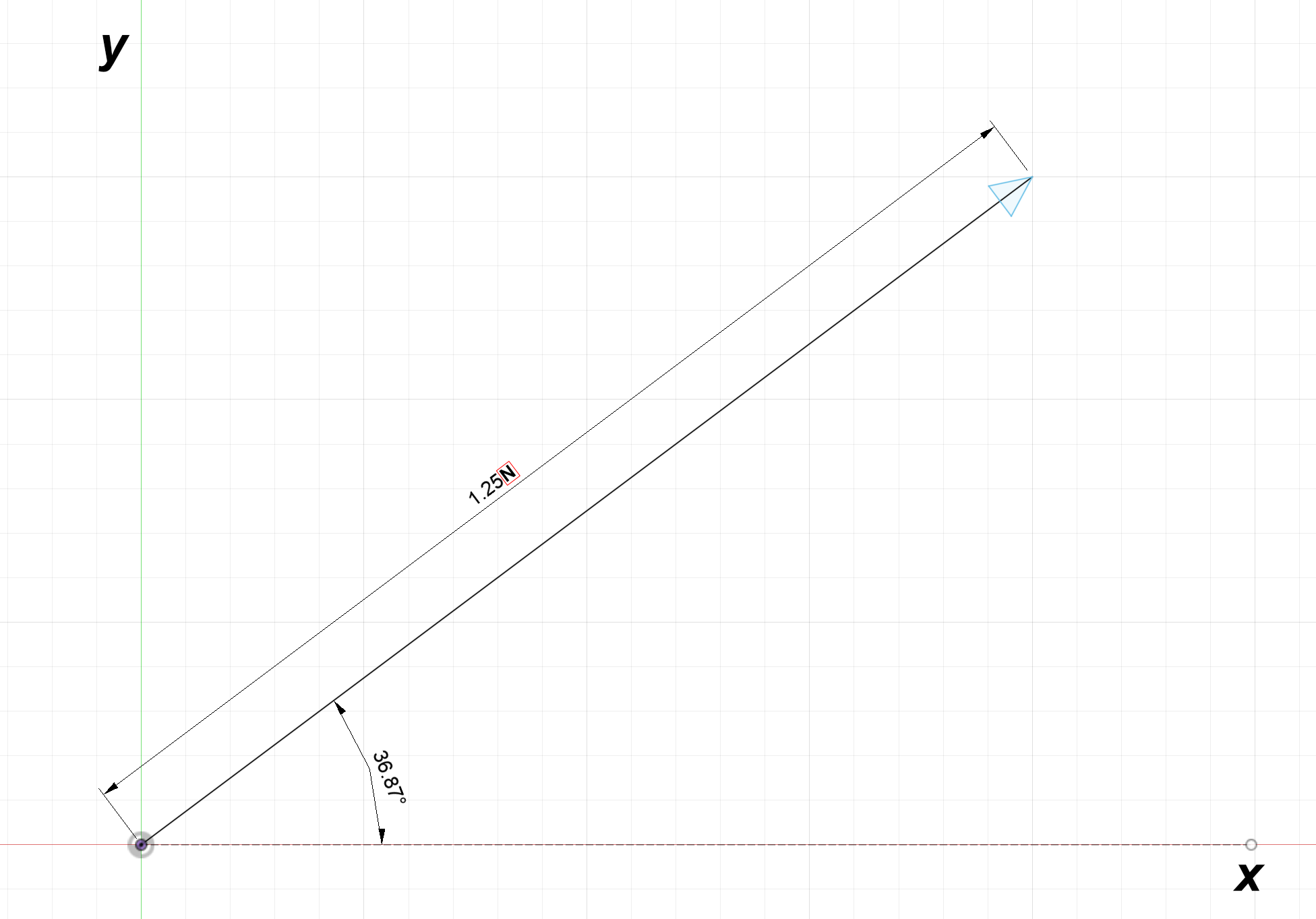
**Figure 2:***Left-* Vector example with units of millimeters per second | *Right-* Vector example with units of newtons

Using the trigonometric functions, any vector can be broken up into components. If you are not familiar with them, I recommend reading the below article.

Suppose the vector in figure 1 is called $\textbf{L}$. We can determine the components of $\textbf{L}$ in the $x$ and $y$ directions. The $x$ component is the adjacent side and the $y$ component is the opposite side:

$L_x = 1.25\text{cos}(36.87^\circ) = 1$

$L_y = 1.25\text{sin}(36.87^\circ) = 0.75$

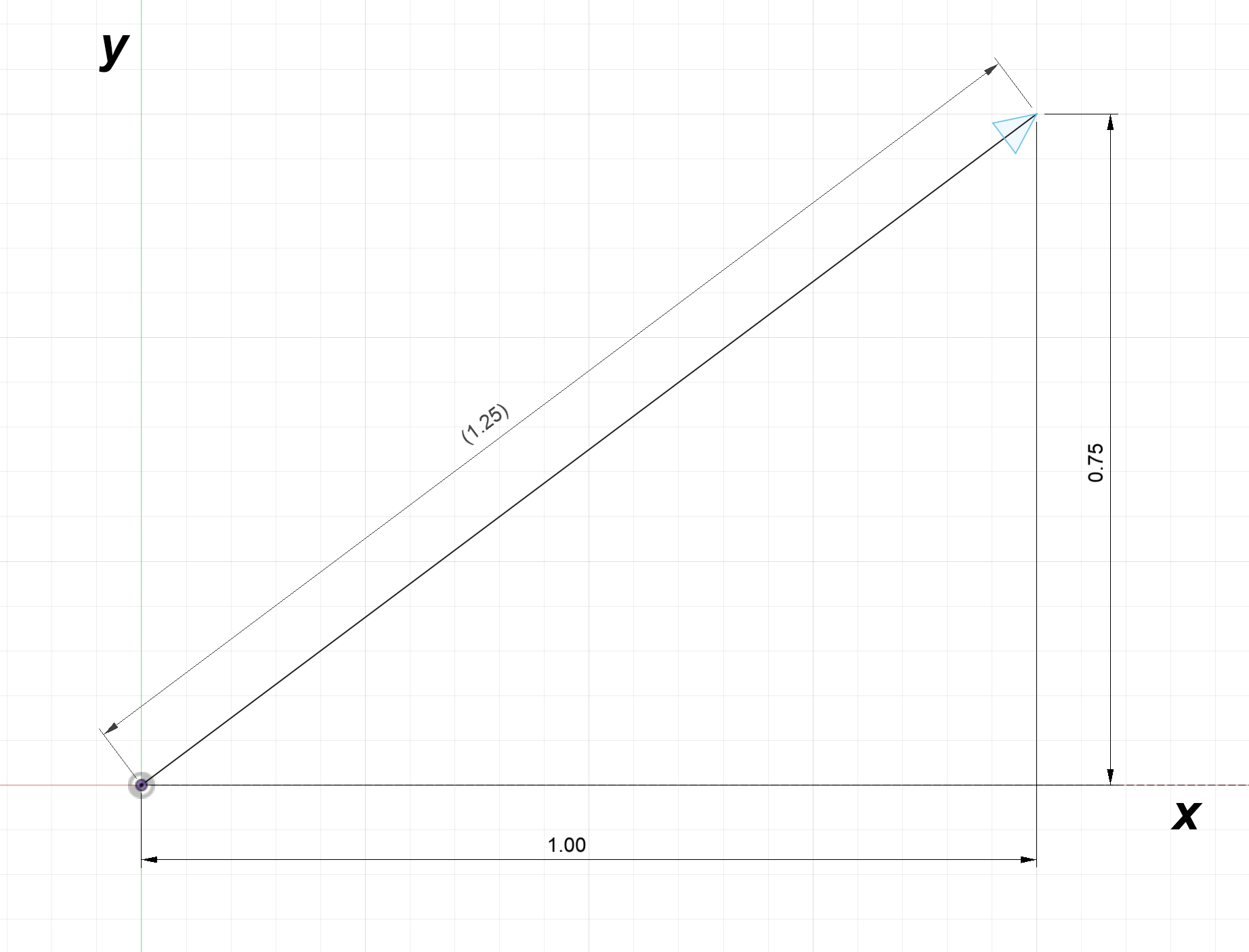
The vector can now be drawn showing its components.

**Figure 3:** Vector example broken into $x$ and $y$ components

This process of splitting a vector into its $x$ and $y$ component is so important that another example is warranted.

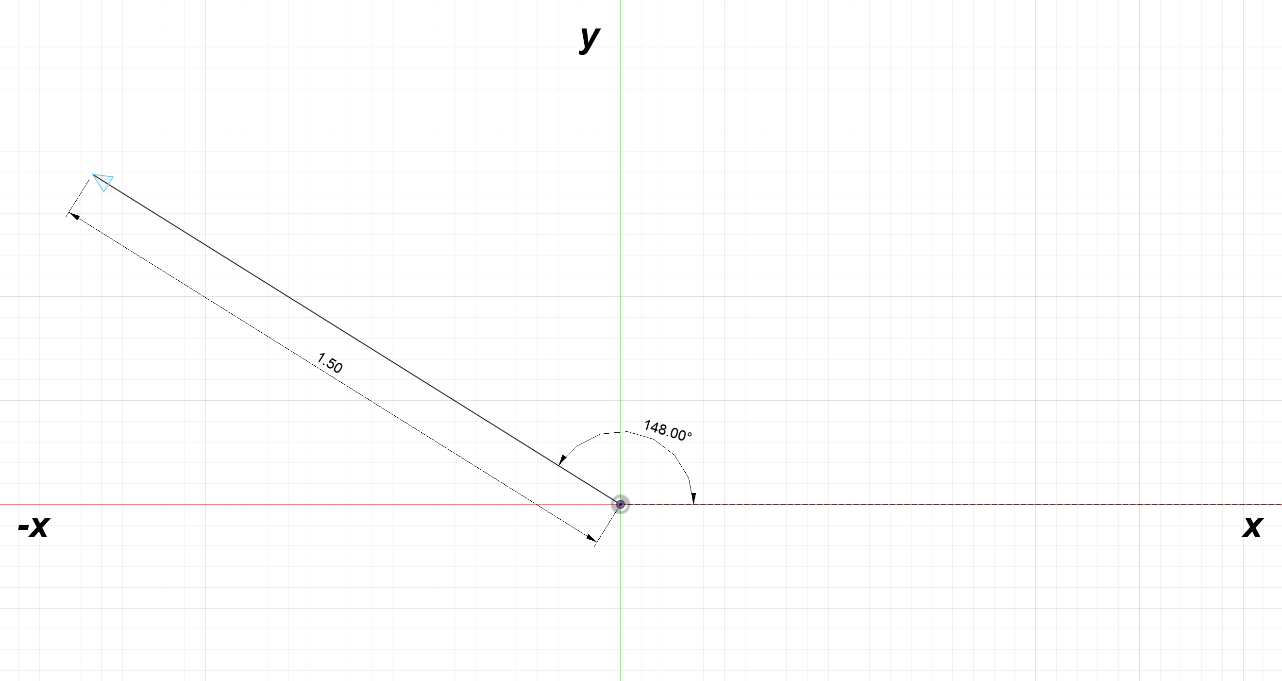
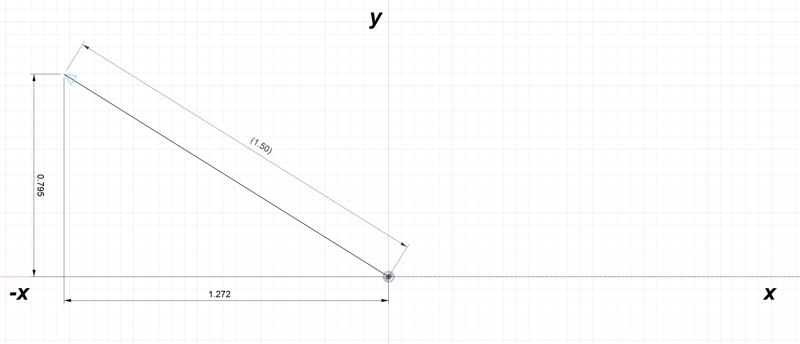
**Figure 4:** Second vector example with $-x$ and $+y$ components

Let's call this second vector $\textbf{L}_2$ and split it into its $x$ and $y$ components:

$L_{2x} = 1.5\text{cos}(148^\circ) = -1.272$

$L_{2y} = 1.5\text{sin}(148^\circ) = 0.795$

**Figure 5:** Second vector example broken into its $-x$ and $+y$ components

Three Dimensional Vectors

Vectors are not limited to two dimensions. Three dimensional vectors are perfectly valid as well.

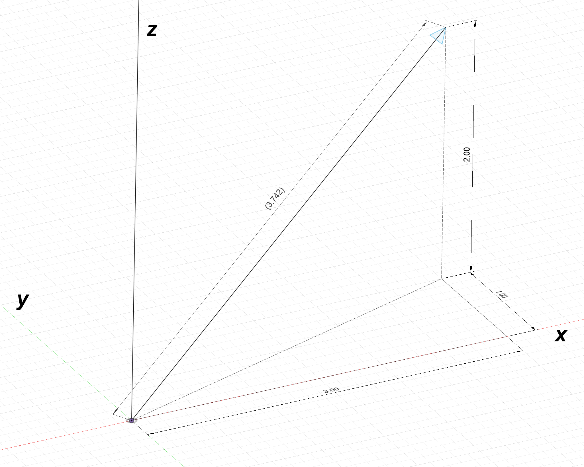
**Figure 6:** Three dimensional vector example broken into $x$, $y$, and $z$ components

The components from the vector in the above diagram are:

$L_x = 3,\:L_y = 1,\:L_z = 2$

$\alpha$, $\beta$, $\gamma$ Representation

One method of describing a 3D vector is by the angles between the vector and the $x$, $y$, and $z$ axes. This is similar to how 2D vectors were first presented in figure 1.

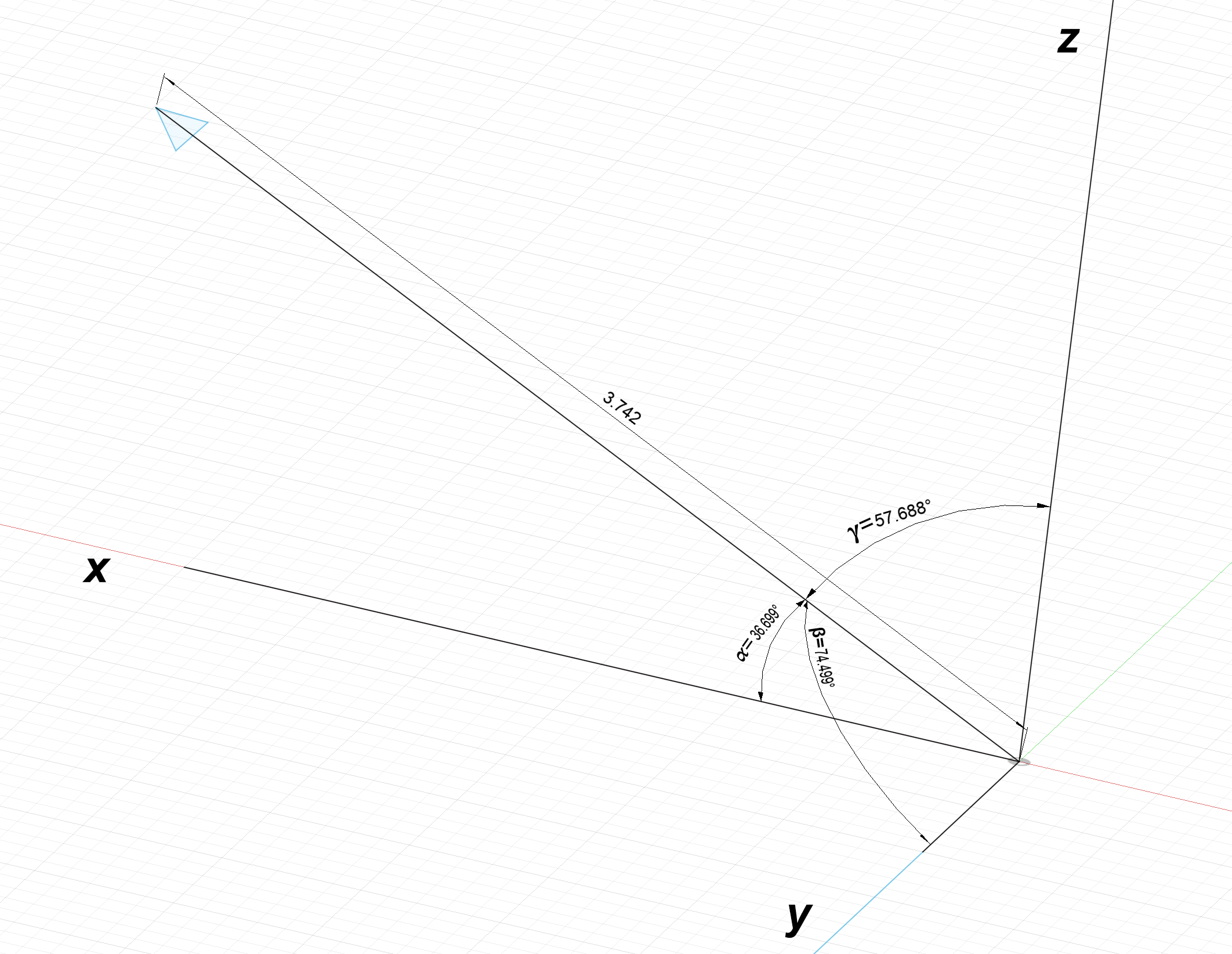
Converting a vector in $\alpha$, $\beta$, $\gamma$ representation to component representation is simple; generate a triangle between each axis and the vector.

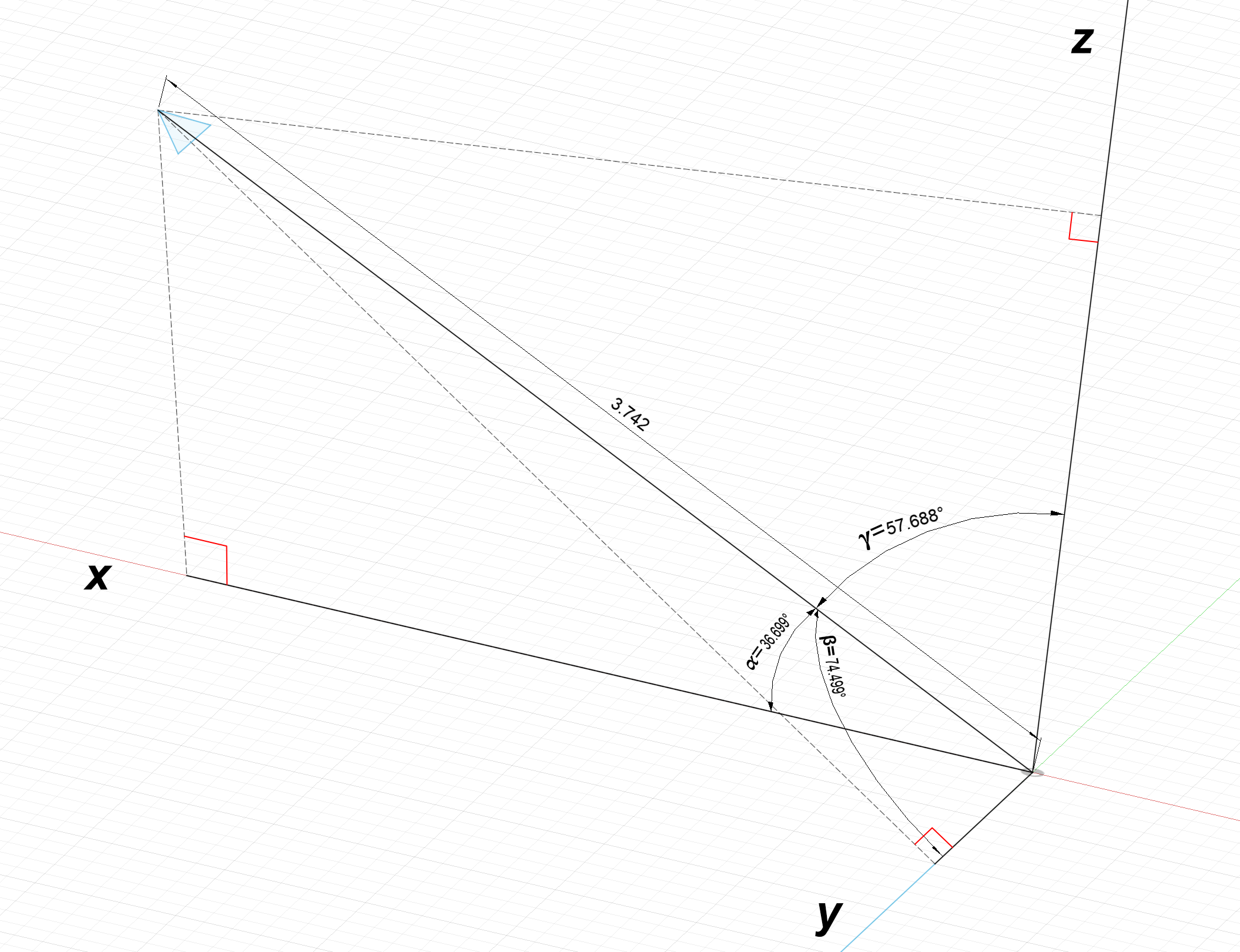
**Figure 8:** $\alpha$, $\beta$, $\gamma$ representation for 3D vector with component triangles

Each component of the vector is the adjacent side of each triangle and can be determined using the cosine function:

$L_x = 3.742\text{cos}(36.699^\circ) = 3$

$L_y = 3.742\text{cos}(57.688^\circ) = 2$

$L_z = 3.742\text{cos}(74.499^\circ) = 1$

$\alpha$, $\beta$ Representation

$\alpha$, $\beta$ representation (not to be confused with $\alpha$, $\beta$, $\gamma$ representation) describes a 3D vector with two angles.

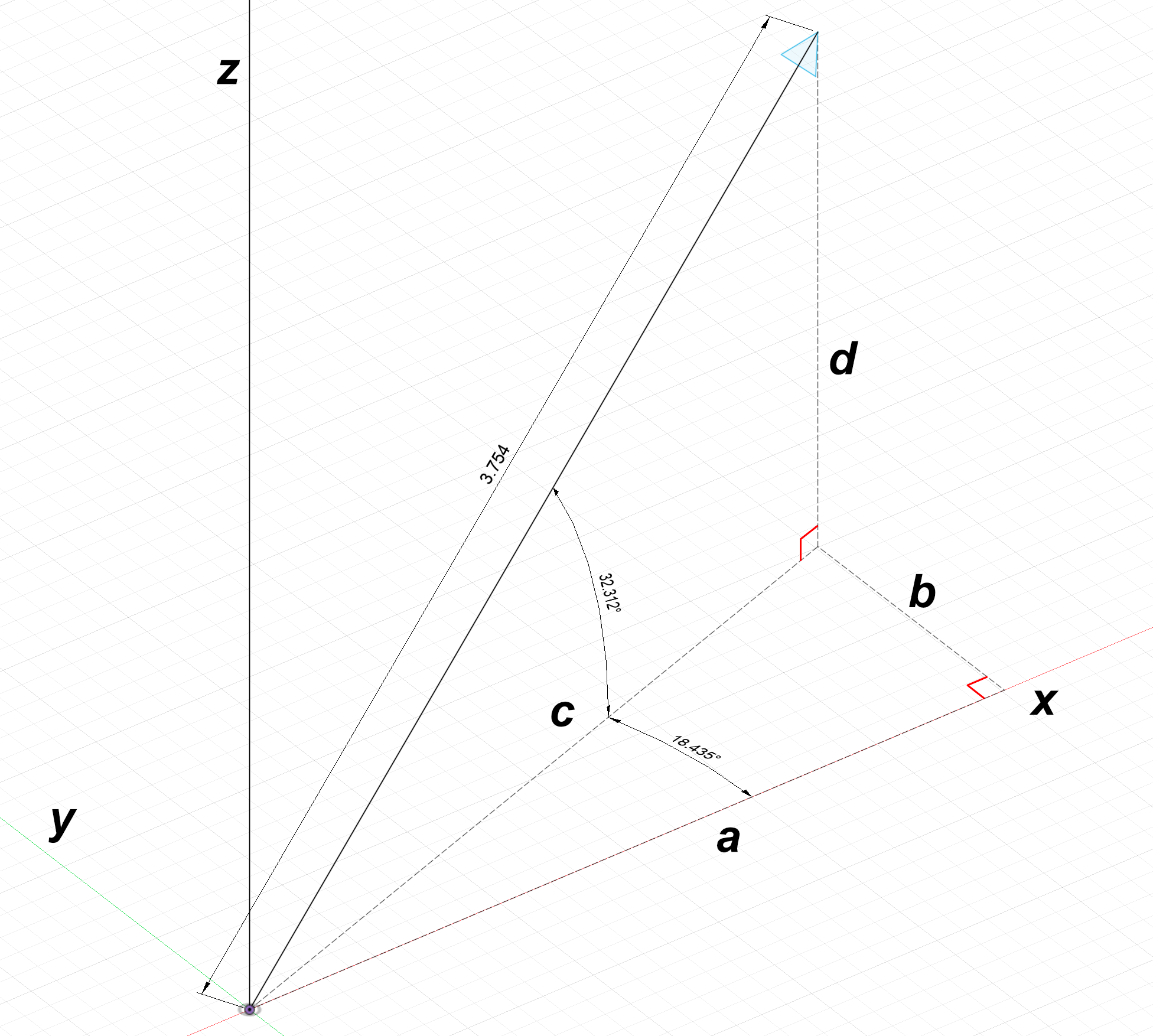
Converting this representation to components is a little more lengthy but still straightforward:

$L_z = d = 3.754\text{sin}(32.312^\circ) = 2$

$c = 3.754 \text{cos}(32.312^\circ) = 3.1726927$

$L_x = a = 3.1726927\text{cos}(18.435^\circ) = 3$

$L_y = b = 3.1726927\text{sin}(18.435^\circ) = 1$

Representing Vectors

It clearly doesn't make sense to represent every vector with a picture and writing multiple equations to describe a vector is a lot of effort. One reasonable method is to represent a vector as a sum of its components. Consider our first vector example, shown below:

**Figure 10:** Vector example broken into $x$ and $y$ components

We can mathematically represent this vector as:

$1 \hat{x} + 0.75 \hat{y}$

Note the use of $x$ and $y$ with little hats on them, $\hat{x}$,$\hat{y}$. These symbols are appropriately called "x-hat" and "y-hat", and they represent the $x$ and $y$ directions. The purpose of using these hatted symbols is because the $x$ and $y$ symbols are often used to represent variables; we want to make sure we don't confuse directions for variables.

We can also represent three dimensional vectors.

**Figure 11:** Three dimensional vector example broken into $x$, $y$, and $z$ components

The above three dimensional vector is represented as:

$3 \hat{x} + 1 \hat{y} + 2 \hat{z}$

A commonly taught alternative to the $\hat{x} $, $\hat{y}$, $\hat{z}$ symbols are $\hat{i} $, $\hat{j}$, and $\hat{k}$ respectively. We might write the above three dimensional vector as:

$3 \hat{i} + 1 \hat{j} + 2 \hat{k}$

I strongly dislike the $\hat{i}$, $\hat{j}$, $\hat{k}$ nomenclature since it conflicts with other symbols we will use in the future. I've shown it here only because it is so often taught.

When referring to something that is a vector, the three most common methods are to make its symbol bold, $\textbf{L}$, to put a line over it, $\overline{L}$, or put an arrow above it, $\overrightarrow{L}$. These are all equivalent.

$\textbf{L} = \overline{L} = \overrightarrow{L} = 3 \hat{x} + 1 \hat{y} + 2 \hat{z}$

On this site, I will generally refrain from using the bold symbol $\textbf{L}$ for vectors and will reserve this for multivectors (described in the Vector Multiplication article).

This method of writing a vector (with each component corresponding to $\hat{x}$, $\hat{y}$, $\hat{z}$) is called the component vector form.

The component vector form has the unfortunate side effect of having to draw a lot of little hats. A much more compact version is the matrix vector form:

$$\overrightarrow{L} = \begin{bmatrix} 3 \\ 1 \\ 2 \end{bmatrix}$$

The first row corresponds to the $\hat{x}$ component, the second to the $\hat{y}$ component, and the third to the $\hat{z}$ component. This is the modern standard vector. A list of numbers set inside brackets.

Vector Positions

While a vector contains magnitude and direction information, it does not contain position information. The below vectors $\overrightarrow{L_1}$ and $\overrightarrow{L_2}$ are equivalent, both equal to $\begin{bmatrix} 1 \\ 1.5 \end{bmatrix}$.

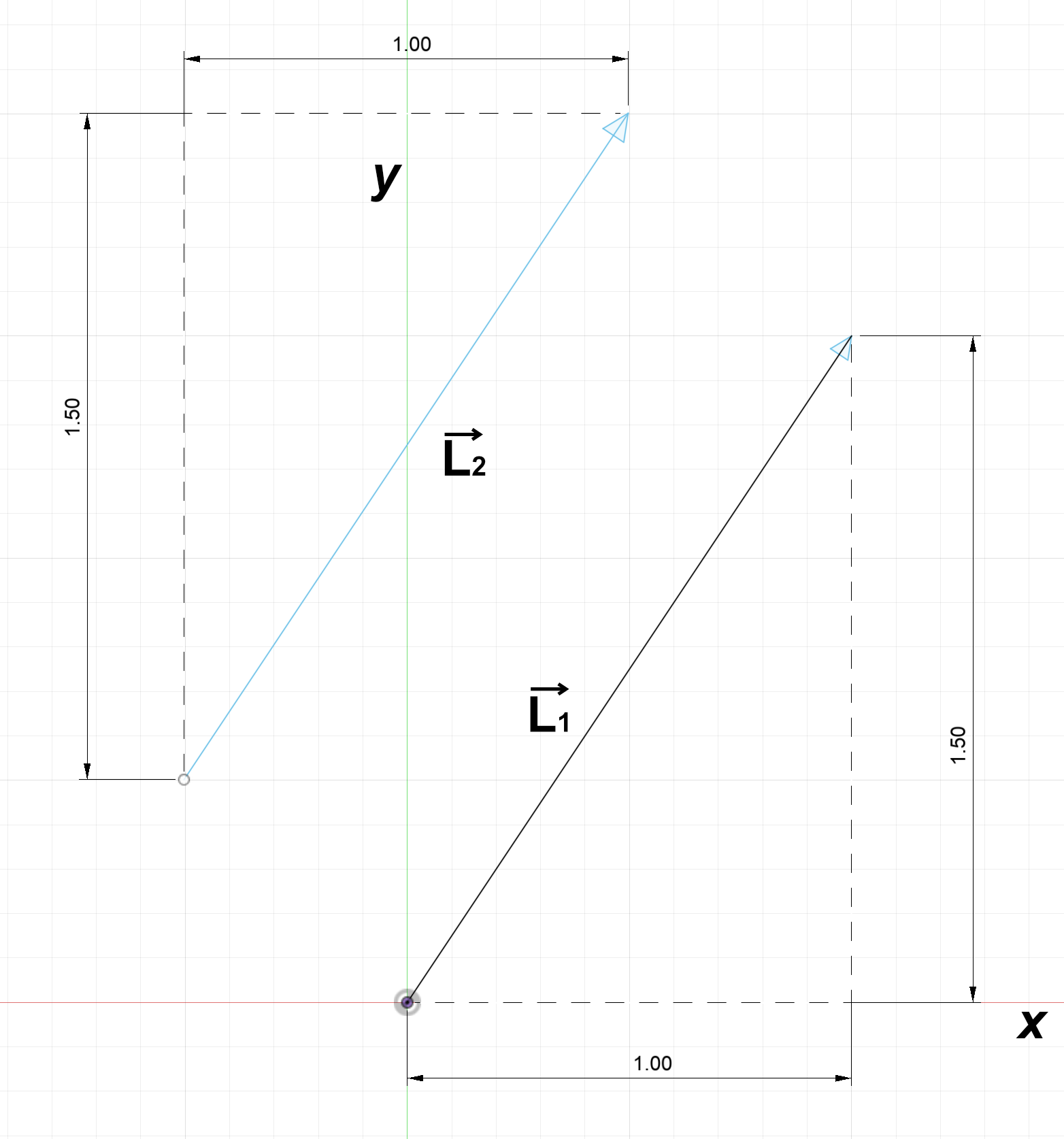
**Figure 12:** Demonstration of vector position independence

To describe the position of a vector requires another vector. The start of vector $\overrightarrow{L_1}$ is located at $\begin{bmatrix} 0 \\ 0 \end{bmatrix}$ while the start of vector $\overrightarrow{L_2}$ is located at $\begin{bmatrix} -0.5 \\ 0.5 \end{bmatrix}$.

Adding and Subtracting Vectors

To add vectors, we put them end to end and add their components.

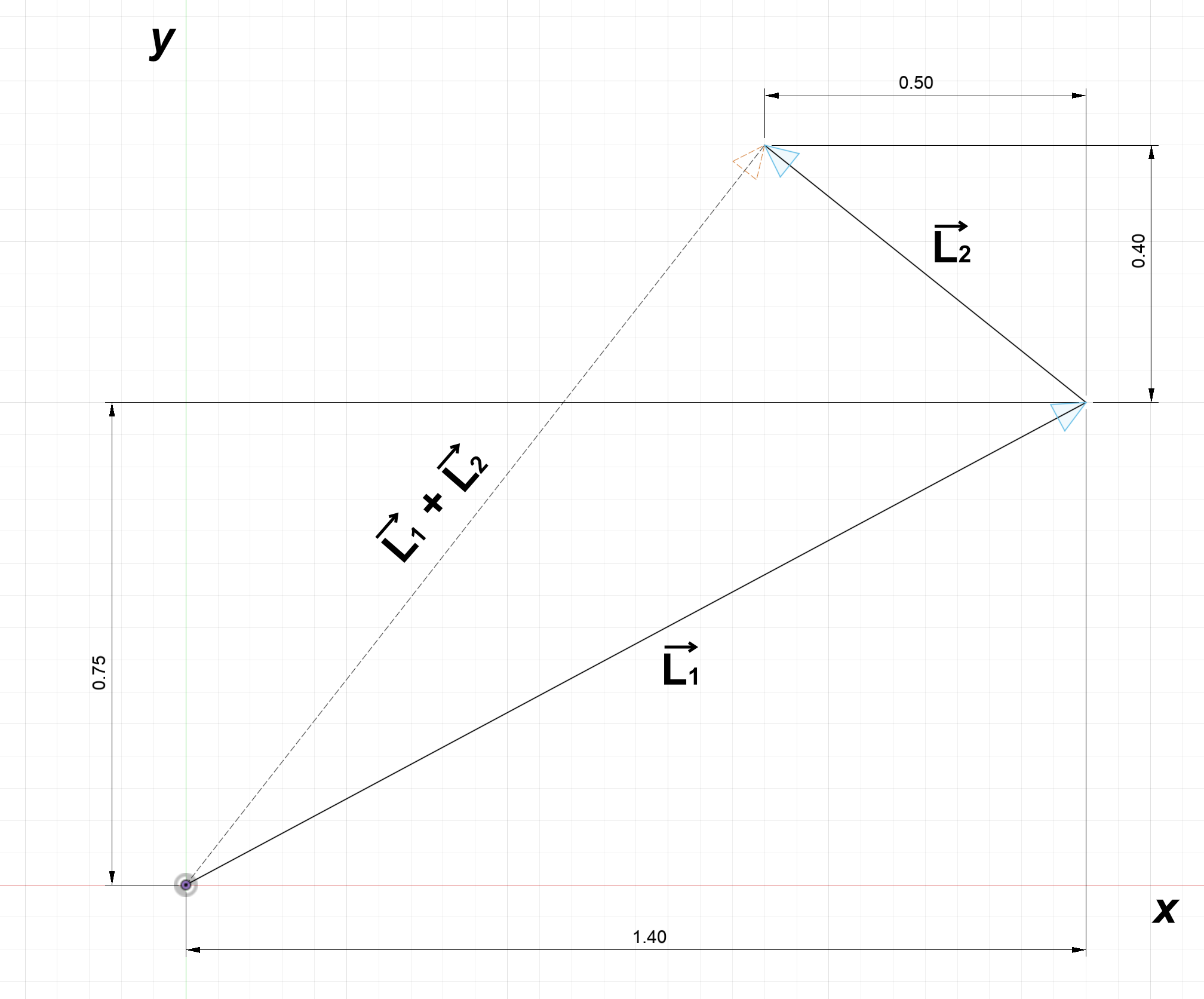
**Figure 13:** Graphical demonstration of vector addition

$$\overrightarrow{L_1} = \begin{bmatrix} 1.4 \\ 0.75 \end{bmatrix},\: \overrightarrow{L_2} = \begin{bmatrix} -0.5 \\ 0.4 \end{bmatrix}$$

$$\overrightarrow{L_1} + \overrightarrow{L_2 } = \begin{bmatrix} 1.4 \\ 0.75 \end{bmatrix} + \begin{bmatrix} -0.5 \\ 0.4 \end{bmatrix} = \begin{bmatrix} 1.4-0.5 \\ 0.75+0.4 \end{bmatrix} = \begin{bmatrix} 0.9 \\ 1.15 \end{bmatrix}$$

To subtract vectors is similar to adding them... except we subtract their components instead of adding them.

$$\overrightarrow{L_1} - \overrightarrow{L_2 } = \begin{bmatrix} 1.4 \\ 0.75 \end{bmatrix} - \begin{bmatrix} -0.5 \\ 0.4 \end{bmatrix} = \begin{bmatrix} 1.4-(-0.5) \\ 0.75-0.4 \end{bmatrix} = \begin{bmatrix} 1.9 \\ 0.35 \end{bmatrix}$$

Lengths and Magnitudes of Vectors

Recall the pythagorean theorem derived in the trigonometric functions article.

$a^2 + b^2 = c^2$

For a two dimensional vector, this equation remains valid. It's magnitude can be calculated by simple substitution.

**Figure 14:** Demonstration of 2D vector magnitude calculation

$c^2 = 1.0^2 + 0.75^2 = 1.5626$

$c = 1.25$

When a vector has units of distance (millimeters, inches, etc.), this quantity is called length. When a vector has other units (speed, acceleration, force, etc.), this quantity is called magnitude.

The symbol for length/magnitude is a set of double vertical bars surrounding the vector. For the above vector $\overrightarrow{L}$, it's length is given by:

$||\overrightarrow{L}|| = 1.25$

The length of a 3D vector is easy to derive.

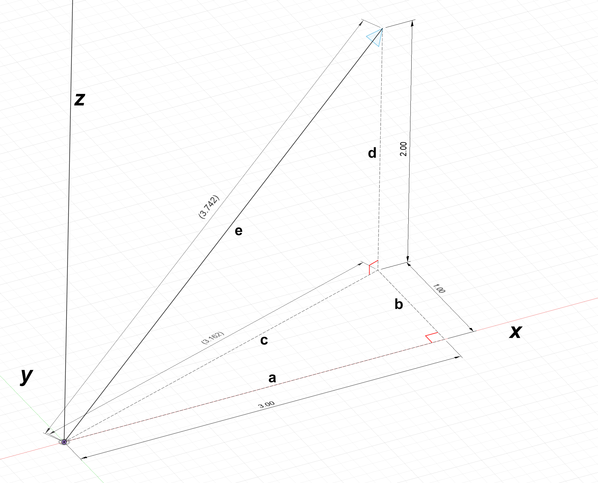
**Figure 15:** Demonstration of 3D vector magnitude calculation

In the diagram above, 3D vector $\textbf{e}$ can be projected onto the $xy$ plane; we can call this projection (which is also a vector) $\textbf{c}$. Note that $a$, $b$, and $d$ are the $x$, $y$, and $z$ components of $\textbf{e}$.

$||\textbf{c}|| = \sqrt{a^2 + b^2} = \sqrt{3^2 + 1^2} = 3.162$

$||\textbf{e}|| = \sqrt{(||\textbf{c}||)^2 + d^2} = \sqrt{3.162^2 + 2^2} = 3.742$

Through symbolic substitution, we can recognize that:

$$(||\textbf{c}||)^2 = a^2 + b^2$$

$$\downarrow$$

$$(||\textbf{e}||)^2 = (||\textbf{c}||)^2 + d^2$$

$$\downarrow$$

$$\boxed{(||\textbf{e}||)^2 = a^2 + b^2 + d^2}$$

This is is the 3D pythagorean theorem; the square of a vector's magnitude is equal to the sum of its components squared. We can apply this formula to obtain the same answer we did earlier though stacked pythagorean theorems:

$$||\textbf{e}|| = \sqrt{a^2 + b^2 + d^2} = \sqrt{3^2 + 1^2 + 2^2} = 3.742$$

Scalars

We've described a vector as a quantity with a direction and magnitude. A scalar is a quantity that is only a magnitude without direction. Every number ($4$, $-73$, $9$, etc.) is a scalar. While vectors are symbolized with a bold symbol $\textbf{L}$ or symbol with an arrow $\overrightarrow{L}$, scalars are represented by regular symbols ($x$, $y$, $\theta$, $\alpha$, etc.).

Scalar Multiplication

When vectors are multiplied by a scalar, they grow in size accordingly. The below diagram shows a vector $\textbf{b}$ which is equal to $2\textbf{a}$.

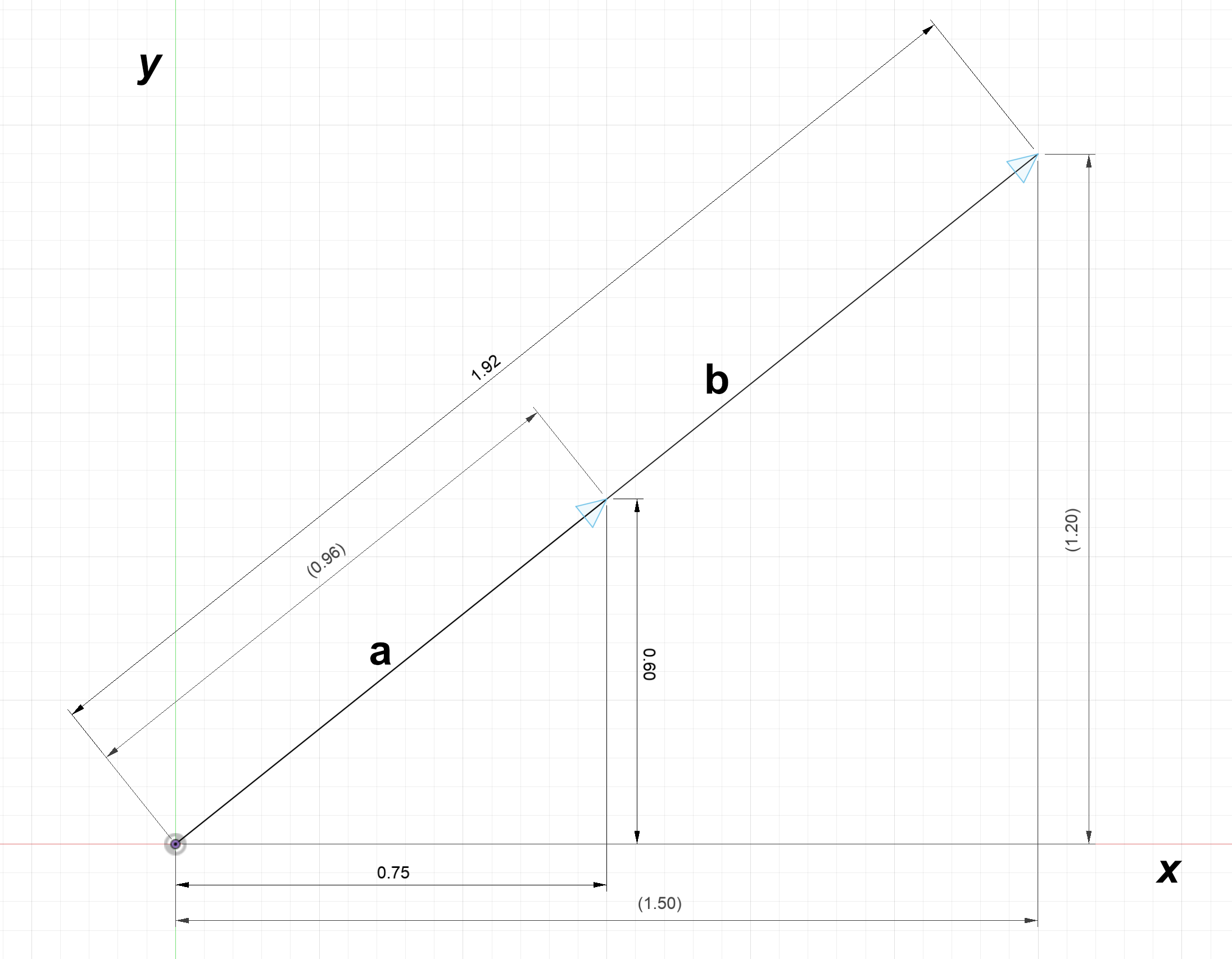
Note that $\textbf{a} = 0.75 \hat{x} + 0.6 \hat{y}$

Multiplying this vector by a scalar is simple:

$2\textbf{a} = 2(0.75 \hat{x} + 0.6 \hat{y}) = 1.5 \hat{x} + 1.2 \hat{y}$

The matrix representation of this is:

$2\textbf{a} = 2\begin{bmatrix} 0.75 \\ 0.6 \end{bmatrix} = \begin{bmatrix} 1.5 \\ 1.2 \end{bmatrix}$

Vector Multiplication

Given the simplicity of scalar multiplication, we might be inclined to attempt multiplication of vectors. Suppose we have two generic vectors:

$\textbf{L}_1 = a \hat{x} + b \hat{y}$

$\textbf{L}_2 = c \hat{x} + d \hat{y}$

Attempting to multiply them together would yield:

$(\textbf{L}_1)(\textbf{L}_2) = (a \hat{x} + b \hat{y})(c \hat{x} + d \hat{y})$

$(\textbf{L}_1)(\textbf{L}_2) = (ac) \hat{x}^2 + (ad)\hat{x}\hat{y} + (bc)\hat{y}\hat{x} + (bd)\hat{y}^2$

What are $\hat{x}^2$, $\hat{x}\hat{y}$, $\hat{y}\hat{x}$, and $\hat{y}^2$!? These are topics for another article, but they are very powerful.