What is Friction?

Prerequisites Required: Forces
In a previous article, we deteremined that Force was the cause for objects to accelerate and deform.

From that article we again use the 3D printed spring and aluminum/plastic blocks to demonstrate properties of friction. Remember that more deflection of the spring means more force was applied to the spring's ends.
For our first experiment, we pull on the spring with our hand.
From this experiment, we focus on the spring's deformation (which measures force) at two key points.
We observe that the spring deforms before the block begins to accelerate. The block is just sitting on the ground! There must be some kind of force acting between the block and the ground that resists acceleration. We call this static friction.

We also observe that the spring continues to remain deformed and transmitting force even when the block is moving at constant velocity (remember, an object in motion should not require force to keep it in motion unless there is some retarding force attempting to slow it down). There must be some kind of force acting between the block and the ground that resists moving at constant velocity. We call this kinetic friction.
Let's repeat the experiment on a plastic block and compare with the aluminum block.

Figure 6-9: Comparison of spring deflection (accelerating and constant velocity) for the plastic and aluminum blocks.
We make two observations based on the stretch of the spring:
- More force is requried to overcome static friction for the aluminum block than the plastic block.
- More force is required to overcome kinetic friction for the aluminum block than for the plastic block.
Thinking about this experiment further, there are many different parameters that might affect the results:
- Does the material of the ground affect friction?
- Does the material of the object affect friction?
- Does the surface texture of the ground affect friction?
- Does the surface texture of the object affect friction?
- Does the mass of the object affect the amount of friction?
- Does the contact area of the surfaces affect friction?
- Does the relative speed between the block and ground affect friction?
Coulomb Friction Model
In 1779, French physicist Charles Augustin de Coulomb published what we now refer to as the Coulomb Friction Model. It is the most commonly taught friction model in introductory physics.
Conceptually, we often think about friction as a force between objects (that may or may not be moving) with imperfect and jagged surfaces (pushed together due to gravity or some other force), as depected in figure 10.
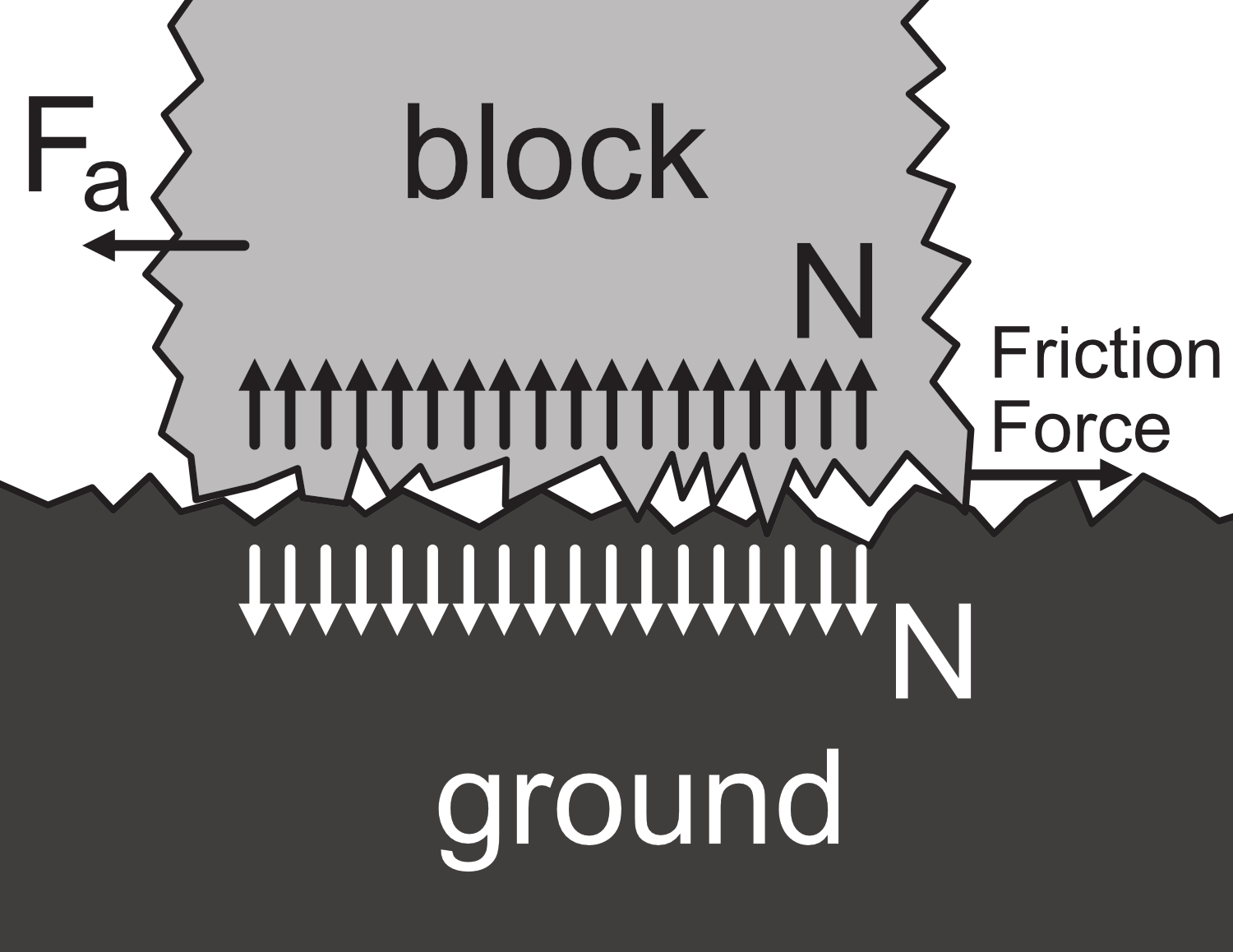
The force that pushes the two objects together is called the normal force because it is oriented perpendicular (normal) to the two contacting surfaces.
The force applied to the block is $F_a$ and the $Friction\:Force$ is the resulting friction force.
Static Friction
For two objects not moving relative to each other ($v = 0$), it takes force to overcome the interlocked jagged surfaces and cause acceleration. The amount of force required to overcome static friction and accelerate an object has a magnitude of:
$$ F_{overcome\:static\:friction} = \mu_sN$$
$N$ is the normal force between the two surfaces. $\mu_s$ is the experimentally determined coefficient of static friction, a value that depends on material and surface texture.
Does surface area affect friction?
In the ideal case, no. In the real world, yes.
We can think of the normal force as distributed over the various peaks of the jagged surface shown in figure 10. The force seen by each of these peaks creates a wedging effect and causes friction.
Suppose a surface contains three peaks. The normal force on each peak is given by:
$$N_p = \frac{N}{3} $$
The force to overcome static friction is then
$$ F_{overcome\:static\:friction} = \mu_sN_p + \mu_sN_p + \mu_sN_p = 3\mu_sN_p$$
We can substitute $N_p = \frac{N}{3}$ into the above equation to find:
$$ F_{overcome\:static\:friction}= 3\mu_sN_p =3\mu_s\frac{N}{3} = \mu_sN$$
Consider now we leave the normal force equal but double the area of the contact surfaces so that the number of peaks is now six. The normal force on each peak is given by:
$$N_p = \frac{N}{6}$$
The force to overcome static friction is then
$$ F_{overcome\:static\:friction} = 6\mu_sN_p$$
We can substitute $N_p = \frac{N}{6}$ into the above equation to find:
$$ F_{overcome\:static\:friction} = 6\mu_sN_p = 6\mu_s\frac{N}{6} = \mu_sN$$
The answer is the same!
In the ideal case, increasing the surface area without increasing the normal force results in each jagged peak seeing less wedging individually, but there are now more jagged peaks that add up such that the friction force is equal.
In the practical case, $\mu_s$ is determined by the contact surfaces themselves and measured in actual experiments.
Deflection due to the normal force, variations in surface texture, and surface physics poorly represented by our simple jagged peak model mean that the friction may not be the same when compared between surfaces with a hundred or thousand fold difference in surface area.
In order for the acceleration to remain zero, the force must be less than the force of static friction, $F_a \le \mu_sN$. This is called the stick-slip criteria. If an applied force is less than the force to overcome static friction, the actual force of friction opposing the applied force is equal and opposite:
$$ F_{static\:friction} = \begin{matrix}-F_a,& F_a \le \mu_sN\:\:\:\&\:\:\: v = 0\end{matrix}$$
If an applied force is greater than the force required to overcome static friction, and the relative surface velocity is zero, the actual force of friction opposing the applied force is equal to:
$$ F_{static\:friction} = \begin{matrix}\mu_sN(-sign(F_a)), & F_a \ge \mu_sN\:\:\:\&\:\:\: v = 0\end{matrix}$$
When this is the case, the object will accelerate.
Kinetic Friction
If two objects are moving relative to each other, the force due to friction is:
$$F_{kinetic\:friction} = \mu_kN(-sign(v)) $$
$N$ is the normal force between the two surfaces. $\mu_k$ is the experimentally determined coefficient of kinetic friction, a value that depends on material and surface texture.
The $sign(v)$ function is the direction of the velocity (positive or negative). The result from $sign(v)$ is negated to indicate that kinetic friction is directed opposite the direction the object is moving; this is a force that causes objects to slow down.
The force from kinetic friction is always less than static friction.
Note that the coulomb friction model does not account for any change in friction due to the relative velocities of the surfaces.
Model Summary
The Coulomb friction model states that for a block with an applied net force, the friction force is:
$$F_{friction} = \left\{\begin{matrix} -F_a, & |F_a| \le \mu_sN \:\: \& \:\: v = 0 \\ \mu_sN(-sign(F_a)), & F_a > \mu_sN\:\: \& \:\: v = 0\\ \mu_kN(-sign(v)), & v \ne 0 \end{matrix} \right.$$
Mathematical Notation Aid (Stacked Conditional Functions)
The above equation is a very compact method of writing the Coulomb friction model. It says that the friction force (shown on the left side) is equal to one of three possible values (shown on the right side). The value for the friction is determined by which of the conditions (shown to the right of the values) are met.
$$F_{friction} = \left\{\begin{matrix} \underbrace{-F_a,}_{value} & \underbrace{|F_a| \le \mu_sN \:\: \& \:\: v = 0}_{condition} \\ \underbrace{\mu_sN(-sign(F_a))}_{value}, & \underbrace{F_a > \mu_sN\:\: \& \:\: v = 0}_{condition}\\ \underbrace{\mu_kN(-sign(v))}_{value}, & \underbrace{v \ne 0}_{condition} \end{matrix} \right.$$
Mathematical Notation Aid (Absolute Value Symbol)
When a number or variable is surrounded by vertical lines, the absolute value or magnitude of that number is denoted. For example:
$$ |-1| = 1$$
$$ |-5| = 5$$
$$ |16| = 16$$
For variables that do not yet have a positive or negative value, a stacked conditional function can be used to evaluate their absolute value:
$$ |a| = \left\{ \begin{matrix} a, & a \ge 0 \\ -a & a < 0 \end{matrix}\right.$$
The Coulomb friction model can be depicted on a graph that shows the relationship between force and velocity (shown below).
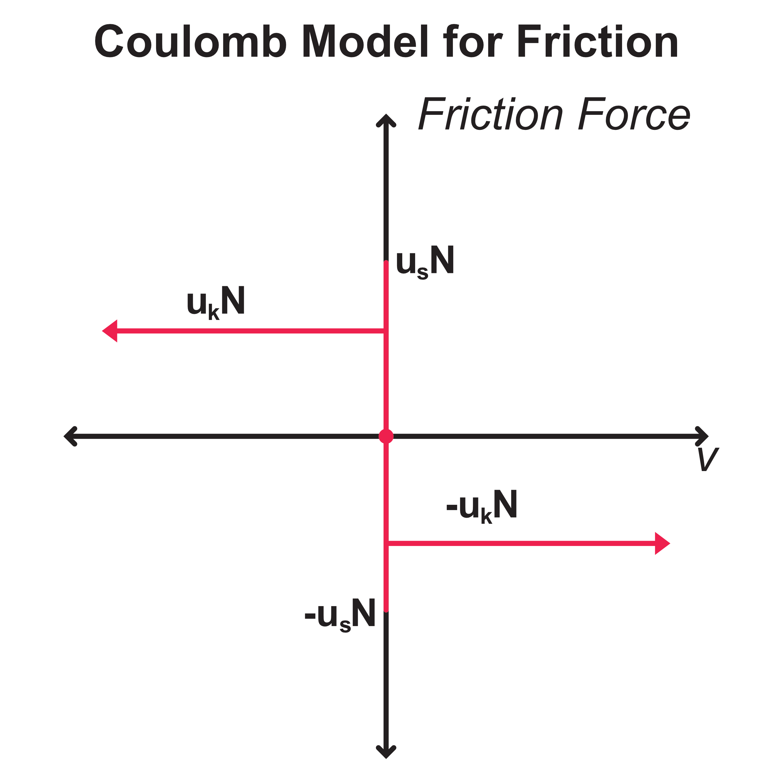
This model works reasonably well when objects are moving at speed and when objects are not moving, but there is a jump discontinuity right at the point of impending acceleration.
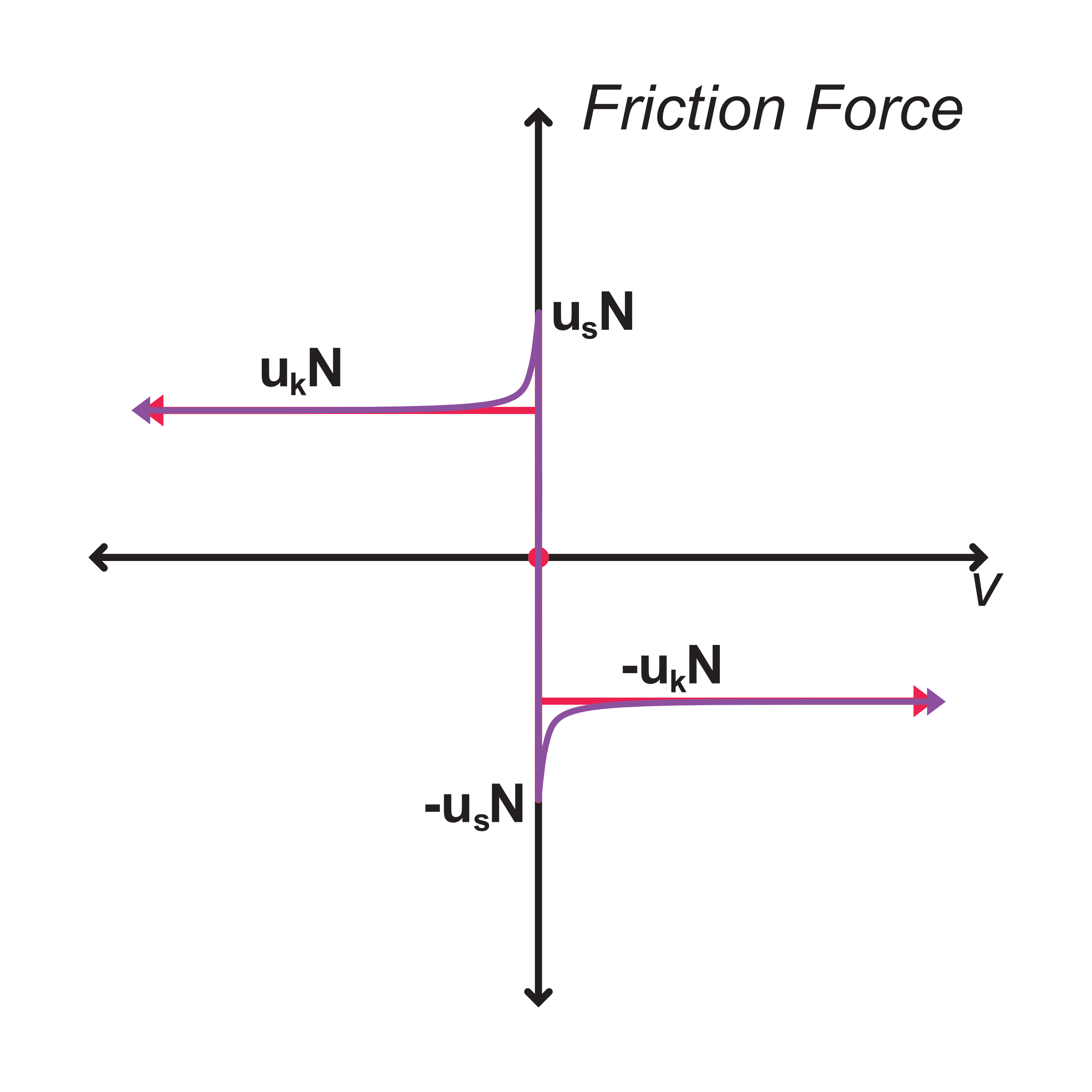
In reality, there is a transition from static to kinetic friction forces as shown in figure 12 below, but it's difficult to measure; the transition occurs very quickly. For most practical situations, there is already so much uncertainty in friction that attempting to model this transition isn't worth the effort it would take.
Viscous Damping Friction Model
The coulomb friction model is typically taught in introductory physics and it works fairly well when modeling a dry contact surface between two rigid objects. However, when deformable objects or wet/lubricated contact surfaces are involved (which happens in pretty much every real machine ever built), we need to consider an additional kind of friction; damping. The force of friction due to damping $F_d$ is proportional to the relative velocity of the two surfaces:
$$ F_d = -cv $$
$c$ is the experimentally determined damping coefficient. $v$ is the relative velocity of the contact surfaces.
The effects of damping are additive with the kinetic friction:
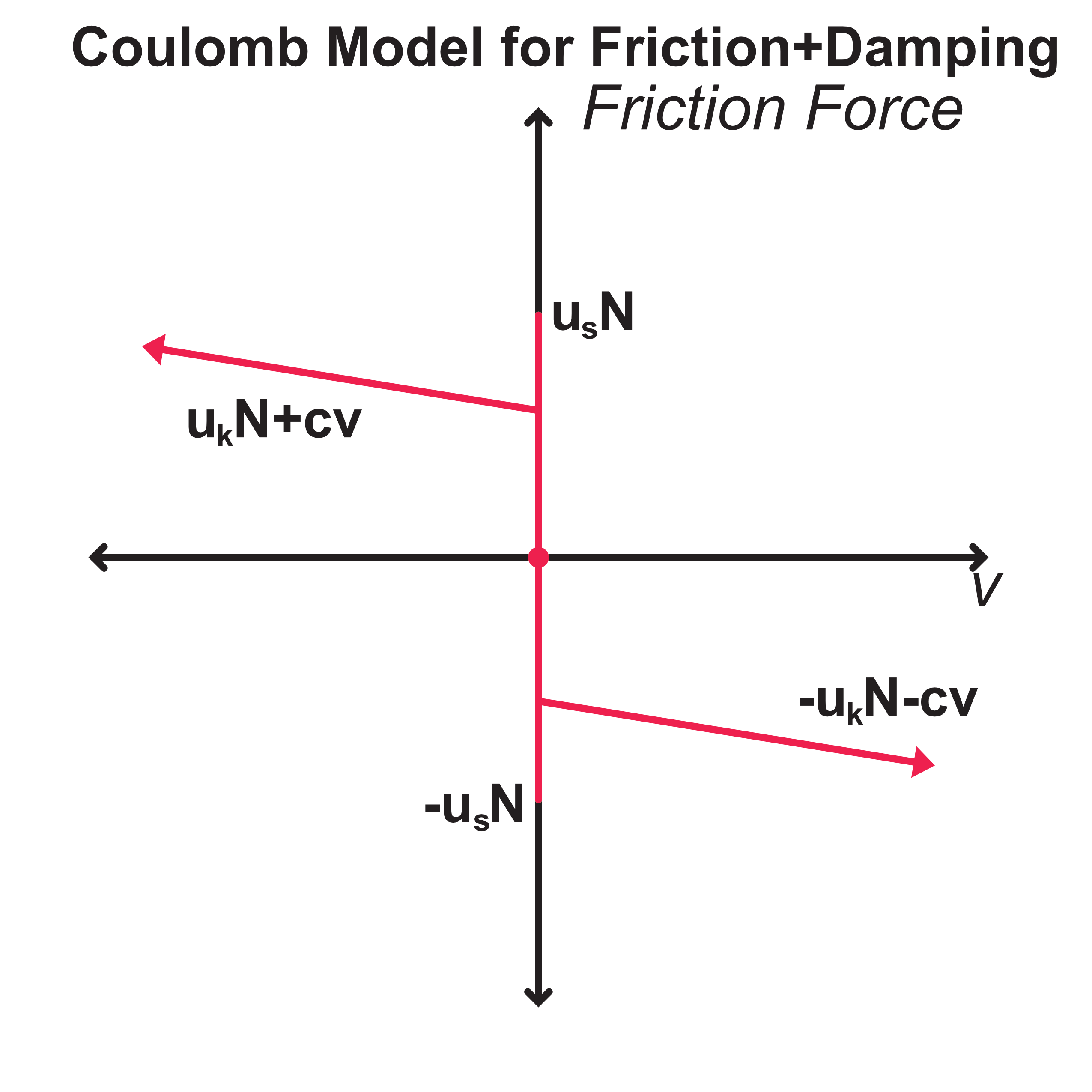
$$F_{friction} = \left\{\begin{matrix} -F_a, & |F_a| \le \mu_sN \:\: \& \:\: v = 0 \\ \mu_sN(-sign(F_a)), & F_a > \mu_sN\:\: \& \:\: v = 0\\ \mu_kN(-sign(v)) - c(v), & v \ne 0 \end{matrix} \right.$$
This is the most common model of friction used by engineers; the enginering model of friction. Like the coulomb friction model, this engineering friction model can also be represented on a graph of force vs velocity.
Other Friction Models
Friction is actually a pretty complicated phenomena. Our models are really just estimations for the material interactions occurring at microscopic scale. The Coulomb and engineering friction models we've discussed so far are common and often successful enough at describing friction to create real machinery, however, not every situation will be well fit by these models.
Some situations require adding a quadratic damping friction term to the model:
$$F_{qd} = bv^2(-sign(v))$$
$$\downarrow$$
$$F_{friction} = \left\{\begin{matrix} -F_a, & |F_a| \le \mu_sN \:\: \& \:\: v = 0 \\ \mu_sN(-sign(F_a)), & F_a > \mu_sN\:\: \& \:\: v = 0\\ \mu_kN(-sign(v)) - c(v) - bv^2(sign(v)), & v \ne 0 \end{matrix} \right.$$
Other friction cases will struggle with the velocity discontinuity between static and kinetic friction. These will need a more sophisticated model.
Some friction cases are so unique that a whole new friction model needs to be created for them.
The validity of a friction model in any situation needs to be tested and verified. Simply assuming a friction model without verification can be a recipe for disaster.
Friction Coefficients
Our engineering friction model involved three different coefficients of friction:
- Coefficient of static friction, $\mu_s$
- Coefficient of kinetic friction, $\mu_k$
- Coefficeint of damping friction, c
You'll notice that I did not tell you what these values are. This was intentional. These values are so situationally dependent on the materials, surface textures, geometries, and lubrication that I do not feel comfortable even giving you recommendations!
There are textual and online resources (just search the internet for "coefficient of friction") where friction coefficients have been determined for a number of materials and geometries. When using these, I recommend extreme caution; these coefficients may or may not be correct for your situation.
Friction coefficients should be experimentaly measured for each situation wherever possible and always validated.